PyTorch官方60分钟教程

PyTorch官方教程

Introduction

What is PyTorch?

PyTorch is a Python-based scientific computing package serving two broad purposes:

• A replacement for NumPy to use the power of GPUs and other accelerators.
• An automatic differentiation library that is useful to implement neural networks.

Goal of this tutorial:

• Understand PyTorch’s Tensor library and neural networks at a high level.
• Train a small neural network to classify images

TENSORS

Tensors 是一种特殊的数据结构，与数组和矩阵非常相似。 在PyTorch中，我们使用Tensors 来编码模型的输入和输出，以及模型的参数。

Tensors 与NumPy的ndarrays类似，除了Tensors 可以在gpu或其他专用硬件上运行以加速计算。 如果你熟悉ndarrays，那么你对Tensors API就很熟悉了。 如果没有，请遵循这个快速的API演练。

import torch
import numpy as np

Tensor Initialization

Tensor 可以用各种方式初始化。 看看下面的例子:

Directly from data

Tensor 可以直接从数据中创建。 数据类型被自动推断出来。

data = [[1, 2], [3, 4]]
x_data = torch.tensor(data)

From a NumPy array

Tensor 可以从NumPy数组中创建(反之亦然——参见Bridge with NumPy)。

np_array = np.array(data)
x_np = torch.from_numpy(np_array)

From another tensor:

新Tensor 保留了参数Tensor 的属性(形状、数据类型)，除非显式地重写。

x_ones = torch.ones_like(x_data) # retains the properties of x_data
print(f"Ones Tensor: \n {x_ones} \n")

x_rand = torch.rand_like(x_data, dtype=torch.float) # overrides the datatype of x_data
print(f"Random Tensor: \n {x_rand} \n")

Out:

Ones Tensor:
 tensor([[1, 1],
        [1, 1]])

Random Tensor:
 tensor([[0.4621, 0.1440],
        [0.6105, 0.6398]])

With random or constant values:

形状是tensor dimensions的元组。 在下面的函数中，它决定了输出tensor的维数。

shape = (2, 3,)
rand_tensor = torch.rand(shape)
ones_tensor = torch.ones(shape)
zeros_tensor = torch.zeros(shape)

print(f"Random Tensor: \n {rand_tensor} \n")
print(f"Ones Tensor: \n {ones_tensor} \n")
print(f"Zeros Tensor: \n {zeros_tensor}")

Out:

Random Tensor:
 tensor([[0.9037, 0.2988, 0.8528],
        [0.9466, 0.9646, 0.3117]])

Ones Tensor:
 tensor([[1., 1., 1.],
        [1., 1., 1.]])

Zeros Tensor:
 tensor([[0., 0., 0.],
        [0., 0., 0.]])

Tensor Attributes

Tensor 属性描述了它们的形状、数据类型和存储它们的设备。

tensor = torch.rand(3, 4)

print(f"Shape of tensor: {tensor.shape}")
print(f"Datatype of tensor: {tensor.dtype}")
print(f"Device tensor is stored on: {tensor.device}")

Out:

Shape of tensor: torch.Size([3, 4])
Datatype of tensor: torch.float32
Device tensor is stored on: cpu

Tensor Operations

超过100个Tensor 操作，包括转置，索引，切片，数学操作，线性代数，随机抽样，以及更多的综合描述在这里。

它们都可以在GPU上运行(通常比在CPU上运行速度更快)。 如果你使用Colab，通过编辑>笔记本设置分配一个GPU

# We move our tensor to the GPU if available
if torch.cuda.is_available():
  tensor = tensor.to('cuda')
  print(f"Device tensor is stored on: {tensor.device}")

Out:

Device tensor is stored on: cuda:0

尝试列表中的一些操作。 如果您熟悉NumPy API，您会发现使用Tensor API很容易。

Standard numpy-like indexing and slicing:

tensor = torch.ones(4, 4)
tensor[:,1] = 0
print(tensor)

Out:

tensor([[1., 0., 1., 1.],
        [1., 0., 1., 1.],
        [1., 0., 1., 1.],
        [1., 0., 1., 1.]])

加入tensors你可以用torch。 将一系列tensors沿给定维数连接起来。

t1 = torch.cat([tensor, tensor, tensor], dim=1)
print(t1)

Out:

tensor([[1., 0., 1., 1., 1., 0., 1., 1., 1., 0., 1., 1.],
        [1., 0., 1., 1., 1., 0., 1., 1., 1., 0., 1., 1.],
        [1., 0., 1., 1., 1., 0., 1., 1., 1., 0., 1., 1.],
        [1., 0., 1., 1., 1., 0., 1., 1., 1., 0., 1., 1.]])

Multiplying tensors

# This computes the element-wise product
print(f"tensor.mul(tensor) \n {tensor.mul(tensor)} \n")
# Alternative syntax:
print(f"tensor * tensor \n {tensor * tensor}")

Out:

tensor.mul(tensor)
 tensor([[1., 0., 1., 1.],
        [1., 0., 1., 1.],
        [1., 0., 1., 1.],
        [1., 0., 1., 1.]])

tensor * tensor
 tensor([[1., 0., 1., 1.],
        [1., 0., 1., 1.],
        [1., 0., 1., 1.],
        [1., 0., 1., 1.]])

它计算两个tensors之间的矩阵乘法

print(f"tensor.matmul(tensor.T) \n {tensor.matmul(tensor.T)} \n")
# Alternative syntax:
print(f"tensor @ tensor.T \n {tensor @ tensor.T}")

​ Out:

tensor.matmul(tensor.T)
 tensor([[3., 3., 3., 3.],
        [3., 3., 3., 3.],
        [3., 3., 3., 3.],
        [3., 3., 3., 3.]])

tensor @ tensor.T
 tensor([[3., 3., 3., 3.],
        [3., 3., 3., 3.],
        [3., 3., 3., 3.],
        [3., 3., 3., 3.]])

具有后缀的操作为就地操作。 例如:x.copy_(y)， x.t_()，将改变x。

print(tensor, "\n")
tensor.add_(5)
print(tensor)

Out:

tensor([[1., 0., 1., 1.],
        [1., 0., 1., 1.],
        [1., 0., 1., 1.],
        [1., 0., 1., 1.]])

tensor([[6., 5., 6., 6.],
        [6., 5., 6., 6.],
        [6., 5., 6., 6.],
        [6., 5., 6., 6.]])

==NOTE:==

就地操作可以节省一些内存，但在计算导数时可能会出现问题，因为会立即丢失历史记录。 因此，不鼓励使用它们

Bridge with NumPy

CPU上的Tensors 和NumPy数组可以共享它们的底层内存位置，改变其中一个就会改变另一个。

Tensor to NumPy array

t = torch.ones(5)
print(f"t: {t}")
n = t.numpy()
print(f"n: {n}")

Out:

t: tensor([1., 1., 1., 1., 1.])
n: [1. 1. 1. 1. 1.]

tensor 的变化反映在NumPy数组中。

t.add_(1)
print(f"t: {t}")
print(f"n: {n}")

Out:

t: tensor([2., 2., 2., 2., 2.])
n: [2. 2. 2. 2. 2.]

NumPy array to Tensor

n = np.ones(5)
t = torch.from_numpy(n)

NumPy数组的变化反映在tensor中。

np.add(n, 1, out=n)
print(f"t: {t}")
print(f"n: {n}")

Out:

t: tensor([2., 2., 2., 2., 2.], dtype=torch.float64)
n: [2. 2. 2. 2. 2.]

A GENTLE INTRODUCTION TO TORCH.AUTOGRAD

torch.autograd是PyTorch的automatic differentiation engine(自动微分引擎) ，为神经网络训练提供动力。 在本节中，您将从概念上理解autograd如何帮助神经网络训练。

Background

神经网络(nns)是一组嵌套函数的集合，在某些输入数据上执行。 这些函数是由参数(由权重和偏差组成)定义的，在PyTorch中，这些参数存储在tensors中。

Training a NN happens in two steps:

Forward Propagation: In forward prop, the NN makes its best guess about the correct output. It runs the input data through each of its functions to make this guess.(在前向支撑中，神经网络对正确的输出进行最佳猜测。 它在每个函数中运行输入数据来进行猜测。)

Backward Propagation: In backprop, the NN adjusts its parameters proportionate to the error in its guess. It does this by traversing backwards from the output, collecting the derivatives of the error with respect to the parameters of the functions (gradients), and optimizing the parameters using gradient descent. For a more detailed walkthrough of backprop, check out this video from 3Blue1Brown.(在背撑模型中，神经网络根据其猜测的误差比例调整参数。 它通过从输出往回遍历，收集关于函数参数(梯度)的误差的导数，并使用梯度下降优化参数来做到这一点。)

Usage in PyTorch

让我们看一下单个训练步骤。 在这个例子中，我们从torchvision中加载了一个预先训练好的resnet18模型。 我们创建一个随机数据张量来表示一个具有3个channels，高度和宽度为64的图像，其对应的标签初始化为一些随机值。 在预先训练的模型中，标签的形状为(1,1000)。

NOTE：本教程只在CPU上工作，不会在GPU上工作(即使张量移动到CUDA)。

import torch, torchvision
model = torchvision.models.resnet18(pretrained=True)
data = torch.rand(1, 3, 64, 64)
labels = torch.rand(1, 1000)

接下来，我们将输入数据在模型的每一层中运行，以做出预测。 这是forward pass。

prediction = model(data) # forward pass

我们使用模型的预测和相应的标签来计算误差(loss)。 下一步是通过网络反向传播此错误。 当我们对error tensor调用. Backward()时，向后传播就开始了。 然后，Autograd在参数的.grad属性中计算并存储每个模型参数的梯度。

loss = (prediction - labels).sum()
loss.backward() # backward pass

接下来，我们加载一个优化器，在本例中，SGD的学习率(learning rate )为0.01，动力(momentum )为0.9。 我们在优化器中注册模型的所有参数。

optim = torch.optim.SGD(model.parameters(), lr=1e-2, momentum=0.9)

最后，我们调用.step()来启动梯度下降。 优化器根据存储在.grad中的梯度来调整每个参数。

optim.step() #gradient descent

现在，您已经具备了训练神经网络所需的一切条件。 下面几节详细介绍了autograd的工作方式——可以跳过它们。

Differentiation in Autograd

让我们看看autograd如何收集梯度。 我们创建了两个tensors a和b，它们的requires_grad=True。 这向autograd发出信号，表示应该跟踪它们上的每个操作。

import torch

a = torch.tensor([2., 3.], requires_grad=True)
b = torch.tensor([6., 4.], requires_grad=True)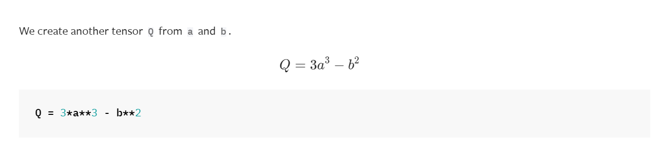

让我们假设“a”和“b”是一个NN的参数，“Q”是误差。 在NN训练中，我们需要误差w.r.t.参数的梯度，即。

$\dfrac{\partial Q}{\partial a} = 9a^2$

$\dfrac{\partial Q}{\partial b} = -2b$

当我们在Q上调用.backward()时，autograd计算这些梯度并将它们存储在各自tensors的.grad属性中。

我们需要在Q.backward()中显式传递一个梯度参数，因为它是一个向量。 梯度是一个与Q形状相同的tensor ，它表示Q w.r.t本身的梯度，即。

$\dfrac{dQ}{dQ} = 1$

同样，我们也可以将Q聚合为标量并隐式地向后调用，如Q.sum().backward()。

external_grad = torch.tensor([1., 1.])
Q.backward(gradient=external_grad)

梯度现在存储在a.grad和b.grad中

# check if collected gradients are correct
print(9*a**2 == a.grad)
print(-2*b == b.grad)

Out:

tensor([True, True])
tensor([True, True])

Optional Reading - Vector Calculus using autograd

数学上，如果你有一个向量值函数 $ \vec{y}=f(\vec{x}) ,$则$ \vec{y}$的梯度关于$ \vec{x}$为雅克比矩阵$ J$

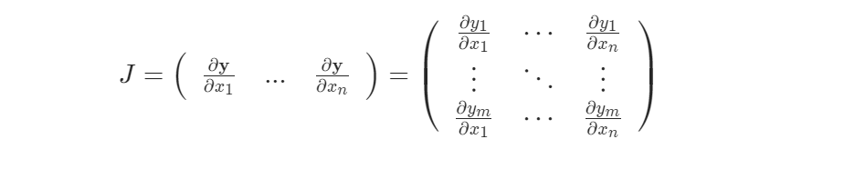
一般来说，$torch.autograd$ 是计算矢量雅克比矩阵乘积的引擎，也就是说，给定任意的向量$\vec{v}$，计算乘积$J^{T}\cdot \vec{v}$

如果 $\vec{v}$是一个标量函数$l=g(\vec{y})$梯度

那么根据链式法则，矢量与雅可比矩阵的乘积将是$l$关于$\vec{x}$的梯度

向量-雅克比矩阵乘积的特点就是我们在上面例子使用的；external_grad 代表$\vec{v}$.

Computational Graph

概念上，autograd在一个由Function对象组成的有向无环图(DAG)中保存数据(tensors)和所有执行的操作(以及产生的新tensors)的记录。在这个DAG中，叶是输入 tensors，根是输出 tensors。 通过从根到叶跟踪这个图，可以使用链式法则自动计算梯度。

在forward pass时，autograd会同时做两件事:

• 运行请求的操作来计算结果tensor，并且
• 在DAG中保持操作的梯度函数。

当在DAG根目录上调用.backward()时，向后传递开始。 autograd:

• 计算每个.grad_fn的梯度，
• 将它们累加到各自张量的.grad属性中，并且
• 利用链式法则，一直传播到leaf tensors。

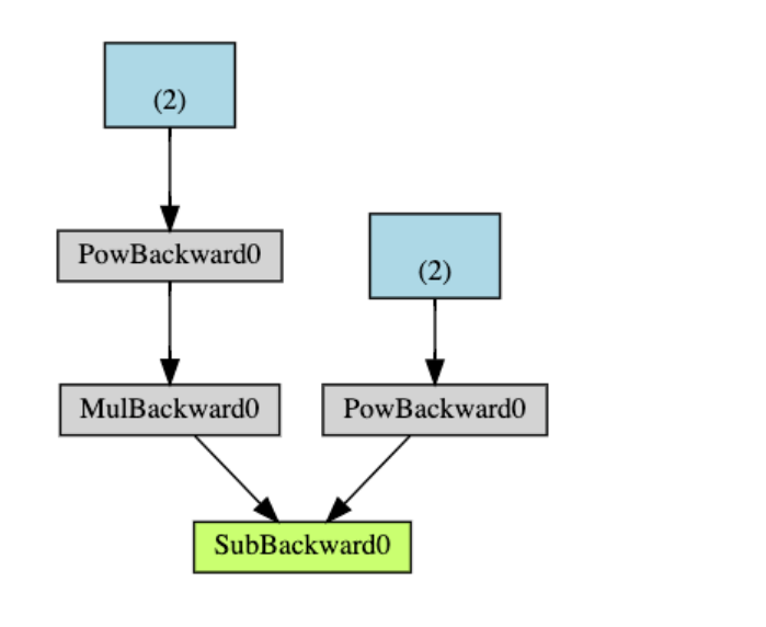
下面是我们示例中的DAG的可视化表示。 在图中，箭头指向forward pass的方向。 节点表示前向传递中每个操作的向后函数。 蓝色的叶节点代表 leaf tensors a和b

NOTE

在PyTorch中，DAGs是动态的,需要注意的重要一点是，图是从头创建的;每次.backward()调用之后，autograd开始填充一个新的图。 这正是允许你在模型中使用控制流语句的原因; 如果需要，您可以在每次迭代中更改形状、大小和操作。

Exclusion from the DAG

torch.autograd tracks operations on all tensors which have their requires_grad flag set to True. For tensors that don’t require gradients, setting this attribute to False excludes it from the gradient computation DAG.

torch.autograd 跟踪所有require_grad标志设置为True的tensors 的操作。 对于不需要梯度的tensors ，将此属性设置为False将其排除在梯度计算DAG中。

操作的输出tensor 将需要梯度，即使只有一个输入tensor 具有requires_grad=True。

x = torch.rand(5, 5)
y = torch.rand(5, 5)
z = torch.rand((5, 5), requires_grad=True)

a = x + y
print(f"Does `a` require gradients? : {a.requires_grad}")
b = x + z
print(f"Does `b` require gradients?: {b.requires_grad}")

在神经网络中，不计算梯度的参数通常称为frozen parameters.。 如果提前知道不需要这些参数的梯度，那么“冻结”模型的一部分是很有用的(这通过减少自动计算提供了一些性能好处)。

从DAG中排除很重要的另一个常见的用例是对预先训练的网络进行微调

在微调中，我们冻结了大部分模型，通常只修改分类器层来预测新标签。 让我们通过一个小示例来演示这一点。 和前面一样，我们加载一个预先训练的resnet18模型，并冻结所有参数。

from torch import nn, optim

model = torchvision.models.resnet18(pretrained=True)

# Freeze all the parameters in the network
for param in model.parameters():
    param.requires_grad = False

假设我们想要在一个有10个标签的新数据集上微调模型。 在resnet中，分类器是最后一个线性层模型。 我们可以简单地用一个新的线性层(默认情况下是解冻的)来替换它，它充当我们的分类器

model.fc = nn.Linear(512, 10)

在模型中的所有参数，除了model.fc的参数冻结。 计算梯度的唯一参数是model.fc的权重和偏差

# Optimize only the classifier
optimizer = optim.SGD(model.parameters(), lr=1e-2, momentum=0.9)

注意，尽管我们在优化器中注册了所有参数，但唯一计算梯度(因此在梯度下降中更新)的参数是分类器的权重和偏差。

在torch.no_grad()中，作为上下文管理器也可以使用相同的排他功能。

NEURAL NETWORKS

Neural networks can be constructed using the package.

神经网络可以用 torch.nn包来构建

Now that you had a glimpse of autograd, nn depends on autograd to define models and differentiate them. An nn.Module contains layers, and a method forward(input) that returns the output.

现在您已经对autograd有了一些了解，nn依赖于autograd来定义模型并区分它们。 一个nn.Module包含层和一个返回输出的forward(input)方法。

例如，看看这个分类数字图像的网络:

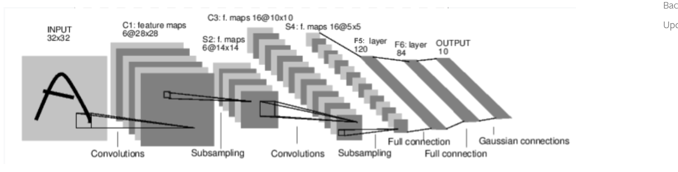
这是一个简单的前馈网络。它接受输入，一个接一个地通过几个层提供输入，最后给出输出。

一个典型的神经网络训练过程如下:

• 定义具有一些可学习参数(或权值)的神经网络
• 迭代输入数据集
• 通过网络处理输入
• 计算损失(输出离正确值有多远)
• 将梯度传播回网络的参数中
• 更新网络的权值，通常使用一个简单的更新规则: weight = weight - learning_rate * gradient

Define the network

Let’s define this network:

import torch
import torch.nn as nn
import torch.nn.functional as F


class Net(nn.Module):

    def __init__(self):
        super(Net, self).__init__()
        # 1 input image channel, 6 output channels, 5x5 square convolution
        # kernel
        self.conv1 = nn.Conv2d(1, 6, 5)
        self.conv2 = nn.Conv2d(6, 16, 5)
        # an affine operation: y = Wx + b
        self.fc1 = nn.Linear(16 * 5 * 5, 120)  # 5*5 from image dimension
        self.fc2 = nn.Linear(120, 84)
        self.fc3 = nn.Linear(84, 10)

    def forward(self, x):
        # Max pooling over a (2, 2) window
        x = F.max_pool2d(F.relu(self.conv1(x)), (2, 2))
        # If the size is a square, you can specify with a single number
        x = F.max_pool2d(F.relu(self.conv2(x)), 2)
        x = torch.flatten(x, 1) # flatten all dimensions except the batch dimension
        x = F.relu(self.fc1(x))
        x = F.relu(self.fc2(x))
        x = self.fc3(x)
        return x


net = Net()
print(net)

Out:

Net(
  (conv1): Conv2d(1, 6, kernel_size=(5, 5), stride=(1, 1))
  (conv2): Conv2d(6, 16, kernel_size=(5, 5), stride=(1, 1))
  (fc1): Linear(in_features=400, out_features=120, bias=True)
  (fc2): Linear(in_features=120, out_features=84, bias=True)
  (fc3): Linear(in_features=84, out_features=10, bias=True)
)

您只需要定义forward函数，backward函数(计算梯度的地方)将使用autograd为您自动定义。 你可以在forward函数中使用任何Tensor 运算。

模型的可学习参数由net.parameters()返回。

params = list(net.parameters())
print(len(params))
print(params[0].size())  # conv1's .weight

Out:

10
torch.Size([6, 1, 5, 5])

让我们尝试一个随机的32x32输入。 注:此网(LeNet)的预期输入大小为32x32。 要在MNIST数据集上使用此网络，请将数据集上的图像大小调整为32x32。

input = torch.randn(1, 1, 32, 32)
out = net(input)
print(out)

Out:

tensor([[-0.0004, -0.0036,  0.0390, -0.0431,  0.0928,  0.1599, -0.0806, -0.0377,
          0.0627, -0.1197]], grad_fn=<AddmmBackward0>)

使用随机梯度将所有参数和后台的梯度缓冲区归零:

net.zero_grad()
out.backward(torch.randn(1, 10))

NOTE

torch.nn 只支持小批量( mini-batches). The entire torch.nn package 只支持小批量样本输入，而不支持单个样本输入。

例如, nn.Conv2d will take in a 4D Tensor of nSamples x nChannels x Height x Width.

如果你只有一个样本，只需使用input.unsqueeze(0)添加一个假的批量尺寸。

在继续之前，让我们回顾一下到目前为止看到的所有类。

Recap:

• torch.Tensor - 一个多维数组，支持像backward()这样的自适应操作。 也保持了tensor的梯度w.r.t。
• nn.Module - 模块-神经网络模块。 封装参数的方便方式，带有将它们移动到GPU、导出、加载等的帮助程序。
• nn.Parameter - tensor的一种，当作为一个属性分配给一个模块时，它会自动注册为一个参数。
• autograd.Function - 函数-实现一个自研操作的向前和向后定义。 每个Tensor操作都至少创建一个函数节点，该节点连接到创建Tensor并编码其历史的函数。

At this point, we covered:

• Defining a neural network
• Processing inputs and calling backward

Still Left:

• Computing the loss
• Updating the weights of the network

Loss Function

loss函数接受(output, target)输入对，并计算一个值来估计输出与目标的距离。

在神经网络包中有几种不同的损失函数。 一个简单的损失是:nn.MSELoss，计算输入和目标之间的均方误差。

For example:

output = net(input)
target = torch.randn(10)  # a dummy target, for example
target = target.view(1, -1)  # make it the same shape as output
criterion = nn.MSELoss()

loss = criterion(output, target)
print(loss)

Out:

tensor(0.8715, grad_fn=<MseLossBackward0>)

现在，如果你使用它的.grad_fn属性向后跟踪loss，你会看到这样的计算图:

input -> conv2d -> relu -> maxpool2d -> conv2d -> relu -> maxpool2d
      -> flatten -> linear -> relu -> linear -> relu -> linear
      -> MSELoss
      -> loss

So, when we call loss.backward(), the whole graph is differentiated w.r.t. the neural net parameters, and all Tensors in the graph that have requires_grad=True will have their .grad Tensor accumulated with the gradient.

因此，当我们调用loss.backward()时，将整个图对神经网络参数w.r.t进行微分，图中所有具有requires_grad=True的Tensors ，其.grad张量将随梯度累加。

为了便于说明，让我们回溯以下几个步骤:

print(loss.grad_fn)  # MSELoss
print(loss.grad_fn.next_functions[0][0])  # Linear
print(loss.grad_fn.next_functions[0][0].next_functions[0][0])  # ReLU

Out:

<MseLossBackward0 object at 0x7fdd1a9f4c18>
<AddmmBackward0 object at 0x7fdd1a9f4940>
<AccumulateGrad object at 0x7fdd1a9f4940>

Backprop

要反向传播错误，我们需要做的就是lose .backward()。 你需要清除现有的梯度，否则梯度将累积到现有的梯度。

现在我们将调用loss.backward()，并查看conv1在向后移动之前和之后的偏移梯度。

net.zero_grad()     # zeroes the gradient buffers of all parameters

print('conv1.bias.grad before backward')
print(net.conv1.bias.grad)

loss.backward()

print('conv1.bias.grad after backward')
print(net.conv1.bias.grad)

Out:

conv1.bias.grad before backward
tensor([0., 0., 0., 0., 0., 0.])
conv1.bias.grad after backward
tensor([ 0.0044,  0.0015, -0.0037, -0.0018, -0.0075,  0.0060])

现在，我们已经知道了如何使用损失函数。

Read Later:

神经网络包包含各种模块和损失函数，构成了深度神经网络的构建块。 这里有一个完整的列表和文档。 here

The only thing left to learn is:

• Updating the weights of the network

Update the weights

The simplest update rule used in practice is the Stochastic Gradient Descent (SGD):

weight = weight - learning_rate * gradient

We can implement this using simple Python code:

learning_rate = 0.01
for f in net.parameters():
    f.data.sub_(f.grad.data * learning_rate)

However, as you use neural networks, you want to use various different update rules such as SGD, Nesterov-SGD, Adam, RMSProp, etc. To enable this, we built a small package: torch.optim that implements all these methods. Using it is very simple:

然而，当您使用神经网络时，您需要使用各种不同的更新规则，如SGD、Nesterov-SGD、Adam、RMSProp等。 为了实现这一点，我们制作了一个小包:torch.optim实现了所有这些方法。 使用它非常简单:

import torch.optim as optim

# create your optimizer
optimizer = optim.SGD(net.parameters(), lr=0.01)

# in your training loop:
optimizer.zero_grad()   # zero the gradient buffers
output = net(input)
loss = criterion(output, target)
loss.backward()
optimizer.step()    # Does the update

NOTE

Observe how gradient buffers had to be manually set to zero using optimizer.zero_grad(). This is because gradients are accumulated as explained in the Backprop section.

观察如何使用optimizer.zero_grad()手动将梯度缓冲区设置为零。 这是因为像Backprop部分所解释的那样，坡度会累积。

TRAINING A CLASSIFIER

This is it。 您已经了解了如何定义神经网络、计算损失和更新网络的权值。

现在你可能会想，

What about data?

通常，当你需要处理图像、文本、音频或视频数据时，你可以使用标准的python包来将数据加载到numpy数组中。 然后你可以把这个数组转换成一个torch.*Tensor.。

• For images, packages such as Pillow, OpenCV are useful
• For audio, packages such as scipy and librosa
• For text, either raw Python or Cython based loading, or NLTK and SpaCy are useful

Specifically for vision, we have created a package called torchvision, that has data loaders for common datasets such as ImageNet, CIFAR10, MNIST, etc. and data transformers for images, viz., torchvision.datasets and torch.utils.data.DataLoader.

特别是对于视觉(vision)，我们创建了一个名为torchvision的包，它拥有用于常见数据集(如ImageNet, CIFAR10, MNIST等)的数据加载器，以及用于图像的数据转换器(如torchvision.datasets和torch.utils.data.DataLoader。

这提供了极大的便利，并避免了编写样板代码。

For this tutorial, we will use the CIFAR10 dataset. It has the classes: ‘airplane’, ‘automobile’, ‘bird’, ‘cat’, ‘deer’, ‘dog’, ‘frog’, ‘horse’, ‘ship’, ‘truck’. The images in CIFAR-10 are of size 3x32x32, i.e. 3-channel color images of 32x32 pixels in size.

在本教程中，我们将使用CIFAR10数据集。 它有类:“飞机”，“汽车”，“鸟”，“猫”，“鹿”，“狗”，“青蛙”，“马”，“船”，“卡车”。 CIFAR-10的图像大小为3x32x32，即32x32像素的3通道彩色图像。

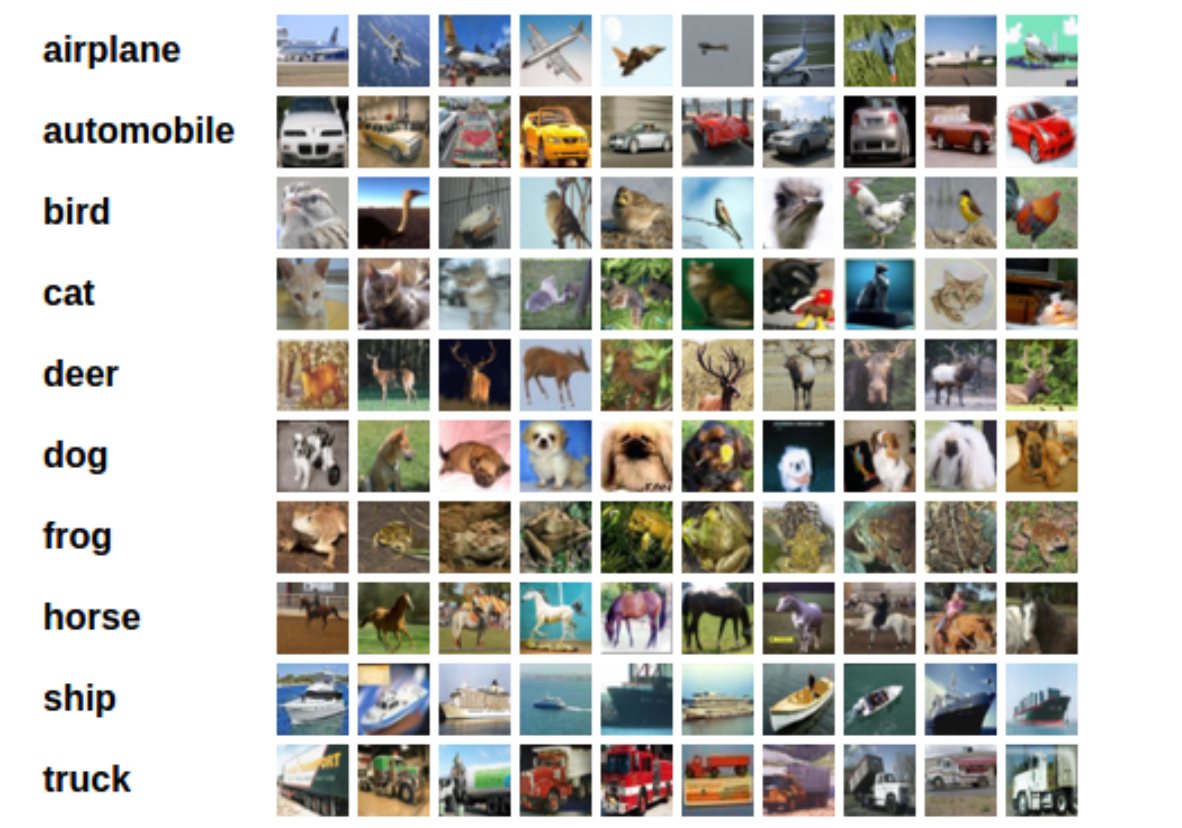
cifar10

Training an image classifier

We will do the following steps in order:

1. Load and normalize the CIFAR10 training and test datasets using torchvision

2. Define a Convolutional Neural Network

3. Define a loss function

4. Train the network on the training data

5. Test the network on the test data

6. Load and normalize CIFAR10

Using torchvision, it’s extremely easy to load CIFAR10.

import torch
import torchvision
import torchvision.transforms as transforms

The output of torchvision datasets are PILImage images of range [0, 1]. We transform them to Tensors of normalized range [-1, 1].

NOTE

If running on Windows and you get a BrokenPipeError, try setting the num_worker of torch.utils.data.DataLoader() to 0.

如果在Windows上运行，你得到一个BrokenPipeError，尝试将torch.utils.data.DataLoader()的num_worker设置为0。

transform = transforms.Compose(
    [transforms.ToTensor(),
     transforms.Normalize((0.5, 0.5, 0.5), (0.5, 0.5, 0.5))])

batch_size = 4

trainset = torchvision.datasets.CIFAR10(root='./data', train=True,
                                        download=True, transform=transform)
trainloader = torch.utils.data.DataLoader(trainset, batch_size=batch_size,
                                          shuffle=True, num_workers=2)

testset = torchvision.datasets.CIFAR10(root='./data', train=False,
                                       download=True, transform=transform)
testloader = torch.utils.data.DataLoader(testset, batch_size=batch_size,
                                         shuffle=False, num_workers=2)

classes = ('plane', 'car', 'bird', 'cat',
           'deer', 'dog', 'frog', 'horse', 'ship', 'truck')

Out:

Downloading https://www.cs.toronto.edu/~kriz/cifar-10-python.tar.gz to ./data/cifar-10-python.tar.gz
Extracting ./data/cifar-10-python.tar.gz to ./data
Files already downloaded and verified

Let us show some of the training images, for fun.

import matplotlib.pyplot as plt
import numpy as np

# functions to show an image


def imshow(img):
    img = img / 2 + 0.5     # unnormalize
    npimg = img.numpy()
    plt.imshow(np.transpose(npimg, (1, 2, 0)))
    plt.show()


# get some random training images
dataiter = iter(trainloader)
images, labels = dataiter.next()

# show images
imshow(torchvision.utils.make_grid(images))
# print labels
print(' '.join(f'{classes[labels[j]]:5s}' for j in range(batch_size)))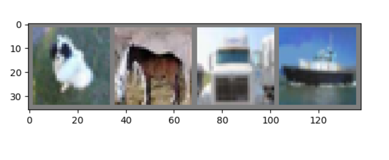

Out:

dog   horse truck ship

2. Define a Convolutional Neural Network

从前面的神经网络部分复制神经网络，并修改它以获取3通道图像(而不是定义的1通道图像)。

import torch.nn as nn
import torch.nn.functional as F


class Net(nn.Module):
    def __init__(self):
        super().__init__()
        self.conv1 = nn.Conv2d(3, 6, 5)
        self.pool = nn.MaxPool2d(2, 2)
        self.conv2 = nn.Conv2d(6, 16, 5)
        self.fc1 = nn.Linear(16 * 5 * 5, 120)
        self.fc2 = nn.Linear(120, 84)
        self.fc3 = nn.Linear(84, 10)

    def forward(self, x):
        x = self.pool(F.relu(self.conv1(x)))
        x = self.pool(F.relu(self.conv2(x)))
        x = torch.flatten(x, 1) # flatten all dimensions except batch
        x = F.relu(self.fc1(x))
        x = F.relu(self.fc2(x))
        x = self.fc3(x)
        return x


net = Net()

3. Define a Loss function and optimizer

Let’s use a Classification Cross-Entropy loss and SGD with momentum.(让我们使用一个分类交叉熵损失和SGD与动量。 )

import torch.optim as optim

criterion = nn.CrossEntropyLoss()
optimizer = optim.SGD(net.parameters(), lr=0.001, momentum=0.9)

4. Train the network

这时候事情开始变得有趣了。 我们只需遍历数据迭代器，将输入输入到网络并进行优化。

for epoch in range(2):  # loop over the dataset multiple times

    running_loss = 0.0
    for i, data in enumerate(trainloader, 0):
        # get the inputs; data is a list of [inputs, labels]
        inputs, labels = data

        # zero the parameter gradients
        optimizer.zero_grad()

        # forward + backward + optimize
        outputs = net(inputs)
        loss = criterion(outputs, labels)
        loss.backward()
        optimizer.step()

        # print statistics
        running_loss += loss.item()
        if i % 2000 == 1999:    # print every 2000 mini-batches
            print(f'[{epoch + 1}, {i + 1:5d}] loss: {running_loss / 2000:.3f}')
            running_loss = 0.0

print('Finished Training')

Out:

[1,  2000] loss: 2.184
[1,  4000] loss: 1.844
[1,  6000] loss: 1.675
[1,  8000] loss: 1.590
[1, 10000] loss: 1.520
[1, 12000] loss: 1.475
[2,  2000] loss: 1.393
[2,  4000] loss: 1.361
[2,  6000] loss: 1.342
[2,  8000] loss: 1.328
[2, 10000] loss: 1.313
[2, 12000] loss: 1.292
Finished Training

Let’s quickly save our trained model:

PATH = './cifar_net.pth'
torch.save(net.state_dict(), PATH)

5. Test the network on the test data

我们对训练数据集进行了2次的训练。 但我们需要检查网络是否了解了什么。

我们将通过预测神经网络输出的类标签来检查这一点，并根据基本事实来检查它。 如果预测是正确的，我们将样本添加到正确的预测列表中。

好的,第一步。 让我们显示一个来自测试集的图像来熟悉一下。

dataiter = iter(testloader)
images, labels = dataiter.next()

# print images
imshow(torchvision.utils.make_grid(images))
print('GroundTruth: ', ' '.join(f'{classes[labels[j]]:5s}' for j in range(4)))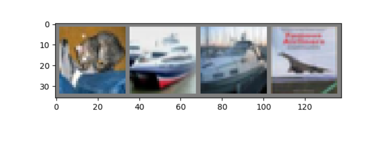

Out:

GroundTruth:  cat   ship  ship  plane

接下来，让我们重新加载已保存的模型(注意:这里并不需要保存和重新加载模型，我们这样做只是为了说明如何做到这一点):

net = Net()
net.load_state_dict(torch.load(PATH))

好了，现在让我们看看神经网络对上面这些例子的看法:

outputs = net(images)

The outputs are energies for the 10 classes. The higher the energy for a class, the more the network thinks that the image is of the particular class. So, let’s get the index of the highest energy:

输出是10类的energies 。 一个类的energy 越高，网络就越认为这个图像是属于这个类的。 那么，让我们得到最高能量的指数:

_, predicted = torch.max(outputs, 1)

print('Predicted: ', ' '.join(f'{classes[predicted[j]]:5s}'
                              for j in range(4)))

Out:

Predicted:  cat   plane ship  plane

结果似乎很好。

让我们看看网络在整个数据集上的表现。

correct = 0
total = 0
# since we're not training, we don't need to calculate the gradients for our outputs
with torch.no_grad():
    for data in testloader:
        images, labels = data
        # calculate outputs by running images through the network
        outputs = net(images)
        # the class with the highest energy is what we choose as prediction
        _, predicted = torch.max(outputs.data, 1)
        total += labels.size(0)
        correct += (predicted == labels).sum().item()

print(f'Accuracy of the network on the 10000 test images: {100 * correct // total} %')

Out:

Accuracy of the network on the 10000 test images: 53 %

这看起来比概率要好得多，后者的准确率是10%(从10个类中随机选出一个类)。 看来网络学到了什么。

嗯，哪些类执行得好，哪些类执行得不好:

# prepare to count predictions for each class
correct_pred = {classname: 0 for classname in classes}
total_pred = {classname: 0 for classname in classes}

# again no gradients needed
with torch.no_grad():
    for data in testloader:
        images, labels = data
        outputs = net(images)
        _, predictions = torch.max(outputs, 1)
        # collect the correct predictions for each class
        for label, prediction in zip(labels, predictions):
            if label == prediction:
                correct_pred[classes[label]] += 1
            total_pred[classes[label]] += 1


# print accuracy for each class
for classname, correct_count in correct_pred.items():
    accuracy = 100 * float(correct_count) / total_pred[classname]
    print(f'Accuracy for class: {classname:5s} is {accuracy:.1f} %')

Out:

Accuracy for class: plane is 73.1 %
Accuracy for class: car   is 61.5 %
Accuracy for class: bird  is 48.2 %
Accuracy for class: cat   is 34.3 %
Accuracy for class: deer  is 37.2 %
Accuracy for class: dog   is 39.8 %
Accuracy for class: frog  is 61.0 %
Accuracy for class: horse is 58.1 %
Accuracy for class: ship  is 76.5 %
Accuracy for class: truck is 43.8 %

好吧，接下来呢?

我们如何在GPU上运行这些神经网络?

Training on GPU

就像你把Tensor 转移到GPU上一样，你把神经网络转移到GPU上。

让我们首先定义我们的设备为第一个可见cuda设备，如果我们有cuda可用:

device = torch.device('cuda:0' if torch.cuda.is_available() else 'cpu')

# Assuming that we are on a CUDA machine, this should print a CUDA device:

print(device)

Out:

cuda:0

本节的其余部分假设该设备是CUDA设备。

然后这些方法将递归地遍历所有模块，并将它们的参数和缓冲区转换为CUDA张量:

net.to(device)

记住，你必须在每一步向GPU发送输入和目标:

inputs, labels = data[0].to(device), data[1].to(device)

为什么我没有注意到与CPU相比的巨大的加速? 因为你们的网络非常小。

练习:尝试增加网络的宽度(第一个nn.Conv2d的参数2)。 和第二个nn.Conv2d的参数1。-它们需要是相同的数字)，看看你得到了什么样的加速。

实现目标:

• 在高水平上理解PyTorch的张量库和神经网络。
• 训练一个小的神经网络来分类图像