python
python中的*与**用法详解
python中*与 **的作用一共有四个,分别是数值计算、序列解包、函数声明的时候作为函数形参、函数调用的时候作为函数实参
序列(列表、元组)解包
list = [1,2,3,4,5]
a,b,*c =list
print('a=',a)
print('b=',b)
print('c=',c)
'''
a= 1
b= 2
c= [3, 4, 5]

'''
list = [1,2]
a,b,*c =list
print('a=',a)
print('b=',b)
print('c=',c)
'''
a= 1
b= 2
c= []
'''
函数声明的时候作为函数形参
大家应该会经常看到类似这样的函数:def function( * arg,** kwargs): ,这里的* arg与**kwarg都是为了接受不定长参数的。其中*arg是位置参数,用于接受不定长的无名参数,本质是一个元组,**kwargs是关键字参数,本质是一个字典。还有一点arg,kwargs就是一个变量名,换成 *a,**b效果是一样的。接下来看代码:
def function(*args,**kwargs):
    print(args)
    print(kwargs)
    print(args[0])
    print(kwargs['b'])
my_list = [1,2,3,'a','b']
my_dict = {'a':1,'b':0,'c':2}
function(*my_list,**my_dict)
- *args 返回的是一个tuple元组- **kwargs返回的是一个dict字典- **kwargs传参只能是A=“B”形式- *args必须要在kwargs前面
def test(*args,**kwargs):
    print(f'args={args}')
    print(f'kwargs={kwargs}')

test(1,2,3,4,food="orange",age=12,sex="F")
dic = {'name':'lisa','job':'nurse'}

结果:
args=(1, 2, 3, 4)
kwargs={'food': 'orange', 'age': 12, 'sex': 'F'}实参分解即将参数拆分成单独的个体
def test(a,b,c):
    print(a)
    print(b)
    print(c)

data1 = ('hello','python','java')
test(*data1)   # 相当于分别传入了3个参数
结果:
a= hello
b= python
c= java

# 此时字典data2的key值必须和形参名称相等,顺序可以不一样
data2 = {'b':'lisa','c':12,'a':'F'}
test(**data2)
结果:
a= F
b= lisa
c= 12
IPython
from IPython import display
The IPython.display module provides a set of functions that can be used to display various types of output in Jupyter notebooks, including images, audio, video, HTML, Markdown, and more.
The display function from the IPython.display module is a particularly useful function, as it allows you to display arbitrary Python expressions in the notebook, and it automatically chooses the appropriate display mechanism based on the type of the expression. For example, you can use display to display the value of a variable, the output of a function call, or even a plot generated by a visualization library.
Here’s an example of how you can use display to show an image in a Jupyter notebook:
from IPython.display import display, Image

# Load the image from a file
image = Image(filename='my_image.png')

# Display the image in the notebook
display(image)
In this example, we first import both the display and Image functions from the IPython.display module. We then load an image from a file using the Image function, and finally we use the display function to show the image in the notebook.
Overall, the IPython.display module and the display function are essential tools for working with Jupyter notebooks, as they make it easy to display a wide variety of output formats directly in the notebook.
pylab
pylab and IPython are two different things in the Python ecosystem.
pylab is a module in the matplotlib library that provides a convenient interface for creating plots and charts in Python. It is essentially a convenience module that provides a simple way to access all of the functionality of matplotlib and numpy in a single namespace. By importing pylab, you get access to a wide range of functionality for creating plots and visualizations, including line plots, scatter plots, histograms, and more.
Here’s an example of how you can use pylab to create a simple line plot:
import pylab

# Create some data
x = [1, 2, 3, 4, 5]
y = [2, 4, 6, 8, 10]

# Create a line plot
pylab.plot(x, y)

# Show the plot
pylab.show()
IPython
On the other hand, IPython is a powerful interactive shell for Python that provides a rich set of tools and features for working with code in an interactive and exploratory way. It is particularly well-suited for working with Jupyter notebooks, which allow you to mix code, text, and visualizations in a single document.
IPython provides a range of useful features for working with Python code interactively, including tab completion, object introspection, and interactive debugging. It also provides a range of useful tools for working with Jupyter notebooks, including support for displaying rich media content (such as images, audio, and video), integrating with third-party libraries, and sharing notebooks with others.
Overall, both pylab and IPython are useful tools for working with Python code, but they serve different purposes. pylab is primarily focused on creating visualizations, while IPython is focused on providing an interactive environment for working with Python code.
常用方法
filter
Python内置的filter()函数能够从可迭代对象(如字典、列表)中筛选某些元素,并生成一个新的迭代器。可迭代对象是一个可以被“遍历”的Python对象,也就是说,它将按顺序返回各元素,这样我们就可以在for循环中使用它。
filter()函数的基本语法是:
filter(function, iterable)一个可迭代的filter对象,可以使用list()函数将其转化为列表,这个列表包含过滤器对象中返回的所有的项。
filter()函数所提供的过滤方法,通常比用列表解析更有效,特别是当我们处理更大的数据集时。例如,列表解析会生成一个新列表,这会增加该处理的运行时间。当列表解析执行完毕它的表达式后,内存中会有两个列表。但是,filter()将生成一个简单的对象,该对象包含对原始列表的引用、提供的函数以及原始列表中位置的索引,这样操作占用的内存更少。
filter()的第一个参数是一个函数,用它来决定第二个参数所引用的可迭代对象中的每一项的去留。此函数被调用后,当返回False时,第二个参数中的可迭代对象里面相应的值就会被删除。针对这个函数,可以是一个普通函数,也可以使用lambda函数,特别是当表达式不那么复杂的时候。
下面是filter()中使用lambda函数的方法:
filter(lambda item: item[] expression, iterable)将下面的列表,用于lambda函数,根据lambda函数表达式筛选列表中的元素。
creature_names = ['Sammy', 'Ashley', 'Jo', 'Olly', 'Jackie', 'Charlie']要筛选此列表以元音开头的水族馆生物的名称,lambda函数如下:
print(list(filter(lambda x: x[0].lower() in 'aeiou', creature_names)))在这里,我们将列表中的一个项声明为x,并以x[0]的方式访问每个字符串的第一个字符,并且要将字母转化为小写,以确保将字母与'aeiou'中的字符匹配。
最后,要提供可迭代对向creature_name。与上一节一样,用list()将返回结果转化为列表表。
输出如下:
['Ashley', 'Olly']当然,写一个函数,也能够实现类似的结果:
creature_names = ['Sammy', 'Ashley', 'Jo', 'Olly', 'Jackie', 'Charlie']

def names_vowels(x):


    return x[0].lower() in 'aeiou'


filtered_names = filter(names_vowels, creature_names)

print(list(filtered_names))在names_vowels函数中用一个表达式,完成了对creature_names的过滤。
同样,输出如下:
['Ashley', 'Olly']总的来说,在filter()函数中使用lambda函数得到的结果与使用常规函数得到的结果相同。如果所要过滤数据更复杂了,还可能要使用正则表达式,这可能会提高代码的可读性。
Map
map是python内置函数,会根据提供的函数对指定的序列做映射。格式是map(function,iterable,...)
第一个参数接受一个函数名,后面的参数接受一个或多个可迭代的序列,返回的是一个集合。
把函数依次作用在list中的每一个元素上,得到一个新的list并返回。注意,map不改变原list,而是返回一个新list。
比如:
del square(x):
    return x ** 2

map(square,[1,2,3,4,5])

# 结果如下:
[1,4,9,16,25]
1234567
还可以实现类型转换 ,比如
map(int,(1,2,3))
# 结果如下:
[1,2,3]

#字符串转list
map(int,'1234')
# 结果如下:
[1,2,3,4]
Reduce
Python 中的 reduce() 函数,它可以用于处理列表。
Python 提供了一个名为 reduce() 的函数,可以更加简洁地实现累积运算。reduce() 函数的语法如下:
reduce(fn,list)reduce() 函数从左至右依次累计使用列表中的元素调用 fn 函数,从而将列表累积生成单个值。
与 map() 和 filter() 函数不同,reduce() 不是 Python 内置函数。实际上,reduce() 函数来自 functools 模块。如果想要使用 reduce() 函数,我们需要在代码开始时使用以下语句导入 functools 模块:
from functools import reduce比如 reduce(lambda x, y: x+y, [1, 2, 3, 4, 5]), 就是计算((((1+2)+3)+4)+5) .
reduce(min,[1,2,6,4,5,])
# 1
reduce(max,[1,2,6,4,5,])
# 6
@staticmethod
@staticmethod是一个Python中的装饰器(decorator),用于标记一个静态方法。
静态方法是一种在类中定义的方法,它与实例无关,因此可以在不创建类实例的情况下调用。与普通方法不同,静态方法没有self参数,因此它不能访问实例属性和方法。
在Python中,使用@staticmethod装饰器可以将一个方法转换为静态方法,即使该方法定义在类中。使用静态方法的主要优点是可以在不创建类实例的情况下调用该方法,从而提高代码的灵活性和可重用性。
下面是一个使用@staticmethod装饰器定义静态方法的示例:
class MyClass:
    @staticmethod
    def my_static_method(x, y):
        return x + y
在上述示例中,my_static_method方法被@staticmethod装饰器标记为静态方法。因此,可以通过以下方式直接调用该方法:
result = MyClass.my_static_method(1, 2)

12
在调用静态方法时,不需要创建类实例,直接使用类名即可。静态方法可以通过类或类实例来调用,但不可以通过实例访问静态方法。
staticmethod相当于定义了一个局部域函数为该类专门服务
lambda
简单用法——隐式函数:
var = lambda a,b : (a + 20) * b
var(20,2)
# 80
var = lambda *a:  [i + 20 for i in a]
var(30,39)
[50, 59]匿名函数lambda:是指一类无需定义标识符(函数名)的函数或子程序。所谓匿名函数,通俗地说就是没有名字的函数,lambda函数没有名字,是一种简单的、在同一行中定义函数的方法。
lambda函数一般功能简单:单行expression决定了lambda函数不可能完成复杂的逻辑,只能完成非常简单的功能。由于其实现的功能一目了然,甚至不需要专门的名字来说明。
lambda 函数可以接收任意多个参数 (包括可选参数) 并且返回单个表达式的值。
lambda表达式只允许包含一个表达式,不能包含复杂语句,该表达式的运算结果就是函数的返回值。
lambda函数实际生成了一个lambda对象。
lambda表达式的基本语法如下:
lambda arg1,arg2,arg3… :<表达式>
arg1/arg2/arg3为函数的参数(函数输入),表达式相当于函数体,运算结果是表达式的运算结果。
例如:
lambda x, y: xy;函数输入是x和y,输出是它们的积xy
lambda:None;函数没有输入参数,输出是None
lambda *args: sum(args); 输入是任意个数的参数,输出是它们的和(隐性要求是输入参数必须能够进行加法运算)
lambda **kwargs: 1;输入是任意键值对参数,输出是1
#测试lambda函数
f=lambda a,b,c,d:a*b*c*d
print(f(1,2,3,4))  #相当于下面这个函数
def test01(a,b,c,d):
    return a*b*c*d
print(test01(1,2,3,4))


g=[lambda a:a*2,lambda b:b*3]
print(g[0](5))  #调用
print(g[1](6))
由于lambda语法是固定的,其本质上只有一种用法,那就是定义一个lambda函数。在实际中,根据这个lambda函数应用场景的不同,可以将lambda函数的用法扩展为以下几种:
1.将lambda函数赋值给一个变量,通过这个变量间接调用该lambda函数。
例如,执行语句add=lambda x, y: x+y,定义了加法函数lambda x, y: x+y,并将其赋值给变量add,这样变量add便成为具有加法功能的函数。例如,执行add(1,2),输出为3。
2.将lambda函数赋值给其他函数,从而将其他函数用该lambda函数替换。
例如,为了把标准库time中的函数sleep的功能屏蔽(Mock),我们可以在程序初始化时调用:time.sleep=lambda x:None。这样,在后续代码中调用time库的sleep函数将不会执行原有的功能。例如,执行time.sleep(3)时,程序不会休眠3秒钟,而是什么都不做。
3.将lambda函数作为参数传递给其他函数。
函数的返回值也可以是函数。例如return lambda x, y: x+y返回一个加法函数。这时,lambda函数实际上是定义在某个函数内部的函数,称之为嵌套函数,或者内部函数。对应的,将包含嵌套函数的函数称之为外部函数。内部函数能够访问外部函数的局部变量,这个特性是闭包(Closure)编程的基础,在这里我们不展开。
部分Python内置函数接受函数作为参数,典型的此类内置函数有这些:
filter函数 此时lambda函数用于指定过滤列表元素的条件。例如filter(lambda x: x % 3 == 0, [1, 2, 3])指定将列表[1,2,3]中能够被3整除的元素过滤出来,其结果是[3]。
sorted函数 此时lambda函数用于指定对列表中所有元素进行排序的准则。例如sorted([1, 2, 3, 4, 5, 6, 7, 8, 9], key=lambda x: abs(5-x))将列表[1, 2, 3, 4, 5, 6, 7, 8, 9]按照元素与5距离从小到大进行排序,其结果是[5, 4, 6, 3, 7, 2, 8, 1, 9]。
map函数 此时lambda函数用于指定对列表中每一个元素的共同操作。例如map(lambda x: x+1, [1, 2,3])将列表[1, 2, 3]中的元素分别加1,其结果[2, 3, 4]。
reduce函数 此时lambda函数用于指定列表中两两相邻元素的结合条件。例如reduce(lambda a, b: ‘{}, {}’.format(a, b), [1, 2, 3, 4, 5, 6, 7, 8, 9])将列表 [1, 2, 3, 4, 5, 6, 7, 8, 9]中的元素从左往右两两以逗号分隔的字符的形式依次结合起来,其结果是’1, 2, 3, 4, 5, 6, 7, 8, 9’。
另外,部分Python库函数也接收函数作为参数,例如gevent的spawn函数。此时,lambda函数也能够作为参数传入。
类型注解
基础
问题
你写好了一个函数,然后想为这个函数的参数增加一些额外的信息,这样的话其他使用者就能清楚的知道这个函数应该怎么使用。
解决方案
使用函数参数注解是一个很好的办法,它能提示程序员应该怎样正确使用这个函数。 例如,下面有一个被注解了的函数:
def add(x:int, y:int) -> int:
    return x + y
python解释器不会对这些注解添加任何的语义。它们不会被类型检查,运行时跟没有加注解之前的效果也没有任何差距。 然而,对于那些阅读源码的人来讲就很有帮助啦。第三方工具和框架可能会对这些注解添加语义。同时它们也会出现在文档中。
>>> help(add)
Help on function add in module __main__:
add(x: int, y: int) -> int
>>>
尽管你可以使用任意类型的对象给函数添加注解(例如数字,字符串,对象实例等等),不过通常来讲使用类或者字符串会比较好点。
语法注意的点:
- 变量类型:在变量名后加一个冒号,冒号后写变量的数据类型,如 int、dict 等
- 函数返回类型:方法参数中如变量类型,在参数括号后加一个箭头,箭头后返回值的类型
- 格式要求(PEP 8,非强制):变量名和冒号无空格,冒号和后边类型间加一个空格,箭头左右均有一个空格
讨论
函数注解只存储在函数的 __annotations__ 属性中。例如:
>>> add.__annotations__
{'y': <class 'int'>, 'return': <class 'int'>, 'x': <class 'int'>}
尽管注解的使用方法可能有很多种,但是它们的主要用途还是文档。 因为python并没有类型声明,通常来讲仅仅通过阅读源码很难知道应该传递什么样的参数给这个函数。 这时候使用注解就能给程序员更多的提示,让他们可以正确的使用函数。
参考9.20小节的一个更加高级的例子,演示了如何利用注解来实现多分派(比如重载函数)。
标准库 typing 类型注解标注
在Python 类型注解中我们介绍过,通过类型注解可以提高代码的可读性和易用性,但对于复杂的数据结构就需要借助 typing 模块来表达这些数据结构。
typing 的作用
Python 类型注解是用来对变量和函数的参数返回值类型做注解(暗示),帮助开发者写出更加严谨的代码,让调用方减少类型方面的错误。
但是,类型注解语法传入的类型表述能力有限,不能说明复杂的类型组成情况,因此引入了 typing 模块,来实现复杂的类型表达。
基础用法
以下是典型的用法:
from typing import List, Tuple, Dict

names: List[str] = ['lily', 'tom']
version: Tuple[int, int, int] = (6, 6, 6)
operations: Dict[str, bool] = {'sad': False, 'happy': True}
安装 mypy 库运行脚本,会强制按类型检测,不符合类型注解要求的会报错:
# 安装
pip install mypy -U
# 运行脚本
mypy program.py
类型
这些是一些最常见的内置类型的示例:
| Type | Description |
|---|---|
| int | 整型 integer |
| float | 浮点数字 |
| bool | 布尔(int 的子类) |
| str | 字符 (unicode) |
| bytes | 8 位字符 |
| object | 任意对象(公共基类) |
| List[str] | 字符组成的列表 |
| Tuple[int, int] | 两个int对象的元组 |
| Tuple[int, …] | 任意数量的 int 对象的元组 |
| Dict[str, int] | 键是 str 值是 int 的字典 |
| Iterable[int] | 包含 int 的可迭代对象 |
| Sequence[bool] | 布尔值序列(只读) |
| Mapping[str, int] | 从 str 键到 int 值的映射(只读) |
| Any | 具有任意类型的动态类型值 |
| Union | 联合类型 |
| Optional | 参数可以为空或已经声明的类型 |
| Mapping | 映射,是 collections.abc.Mapping 的泛型 |
| MutableMapping | Mapping 对象的子类,可变 |
| Generator | 生成器类型, Generator[YieldType、SendType、ReturnType] |
| NoReturn | 函数没有返回结果 |
| Set | 集合 set 的泛型, 推荐用于注解返回类型 |
| AbstractSet | collections.abc.Set 的泛型,推荐用于注解参数 |
| Sequence | collections.abc.Sequence 的泛型,list、tuple 等的泛化类型 |
| TypeVar | 自定义兼容特定类型的变量 |
| Generic | 自定义泛型类型 |
| NewType | 声明一些具有特殊含义的类型 |
| Callable | 可调用类型, Callable[[参数类型], 返回类型] |
Any 类型和类型构造函数如 List,Dict,Iterable 和 Sequence 定义了类型模型。
Dict 类型是一个通用类,由 […] 中的类型参数表示。 如 Dict[int,str] 是从整数到字符串的字典,而 Dict[Any, Any] 是动态键入(任意)值和键的字典。 List 是另一个通用类。 Dict 和 List 分别是内置 dict 和 list 的别名。
Iterable、Sequence 和 Mapping 是与 Python 协议相对应的通用类型。 例如,当期望 Iterable[str] 或 Sequence[str] 时,str 对象或 List[str] 对象有效。 请注意,尽管它们类似于 collections.abc(以前的collections)中定义的抽象基类,但它们也不相同,因为内置的collection 类型对象不支持索引。
变量
Python 3.6 在 PEP 526 中引入了用于注释变量的语法,我们在大多数示例中都使用了它。
# 声明变量类型的类型的方式,python 3.6 +
age: int = 1
# 在 Python 3.5 及更低版本中,您可以改用类型注释
# 同上效果
age = 1  # type: int
# 无需初始化变量即可对其进行注释
a: int  # ok(但不能调用,name 'a' is not defined,直到被赋值)
# 在条件分支中很有用
child: bool
if age < 18:
    child = True
else:
    child = False
内置类型
typing 内置的一些类型的用法:
from typing import List, Set, Dict, Tuple, Optional

# 对于简单的 Python 内置类型,只需使用类型的名称
x: int = 1
x: float = 1.0
x: bool = True
x: str = "test"
x: bytes = b"test"
# 对于 collections ,类型名称用大写字母表示,并且
# collections 内类型的名称在方括号中
x: List[int] = [1]
x: Set[int] = {6, 7}
# 与上述相同,但具有类型注释语法
x = [1]  # type: List[int]
# 对于映射,需要键和值的类型
x: Dict[str, float] = {'field': 2.0}
# 对于固定大小的元组,指定所有元素的类型
x: Tuple[int, str, float] = (3, "yes", 7.5)
# 对于可变大小的元组,使用一种类型和省略号
x: Tuple[int, ...] = (1, 2, 3)
# 使用 Optional[] 表示可能为 None 的值
x: Optional[str] = some_function()
# Mypy 理解 if 语句中的值不能为 None
if x is not None:
    print(x.upper())
# 如果由于某些不变量而使值永远不能为 None,请使用断言
assert x is not None
print(x.upper())
函数
Python 3 支持函数声明的注释语法。
from typing import Callable, Iterator, Union, Optional, List

# 注释函数定义的方式
def stringify(num: int) -> str:
    return str(num)

# 指定多个参数的方式
def plus(num1: int, num2: int) -> int:
    return num1 + num2

# 在类型注释后为参数添加默认值
def f(num1: int, my_float: float = 3.5) -> float:
    return num1 + my_float

# 注释可调用(函数)值的方式, lambda 可以此方法
x: Callable[[int, float], float] = f

# 产生整数的生成器函数安全地返回只是一个
# 整数迭代器的函数,因此这就是我们对其进行注释的方式
def g(n: int) -> Iterator[int]:
    i = 0
    while i < n:
        yield i
        i += 1

# 可以将功能注释分成多行
def send_email(address: Union[str, List[str]],
               sender: str,
               cc: Optional[List[str]],
               bcc: Optional[List[str]],
               subject='',
               body: Optional[List[str]] = None
               ) -> bool:
    ...
混杂结构
以下是一些复杂结构的用法:
from typing import Union, Any, List, Optional, cast

# Union 表示可能是以下几种类型
x: List[Union[int, str]] = [3, 5, "test", "fun"]

# 不知道类型或它太动态而无法为它编写类型,请使用 Any
x: Any = mystery_function()

# 如果使用空容器或“无”初始化变量
# 类型注解帮助 mypy 获知类型信息
x: List[str] = []
x: Optional[str] = None

# 每个位置 arg 和每个关键字 arg 均为 str
def call(self, *args: str, **kwargs: str) -> str:
    request = make_request(*args, **kwargs)
    return self.do_api_query(request)

# cast 可以转换类型
a = [4]
b = cast(List[int], a)  # 正常通过
c = cast(List[str], a)  # 正常通过 (运行是不做检查,无影响)

# 如果要在类上使用动态属性,请使其覆盖 “ __setattr__”
# 或 “ __getattr__”。
#
# "__setattr__" 允许动态分配名称
# "__getattr__" 允许动态访问名称
class A:
    # 如果 x 与“值”属于同一类型,则这将允许分配给任何 A.x
    # (使用“value: Any”以允许任意类型)
    def __setattr__(self, name: str, value: int) -> None: ...

    # 如果 x 与返回类型兼容,则将允许访问任何 A.x
    def __getattr__(self, name: str) -> int: ...

a.foo = 42  # Works
a.bar = 'Ex-parrot'  # Fails type checking
用户定义的泛型类型
用户定义的类可以定义为泛型类。
from typing import TypeVar, Generic
from logging import Logger

T = TypeVar('T')

class LoggedVar(Generic[T]):
    def __init__(self, value: T, name: str, logger: Logger) -> None:
        self.name = name
        self.logger = logger
        self.value = value

    def set(self, new: T) -> None:
        self.log('Set ' + repr(self.value))
        self.value = new

    def get(self) -> T:
        self.log('Get ' + repr(self.value))
        return self.value

    def log(self, message: str) -> None:
        self.logger.info('%s: %s', self.name, message)
Generic[T] 是定义类 LoggedVar 的基类,该类使用单类型参数 T。在该类体内,T 是有效的类型。
lambda 的类型标注
由于类型注解的语法和 lambda 的语法冲突,因此不能直接对 lambda 做类型注解,但我们可以将 lambda 传给一个变量,通过对这个变量做 lambda,达到相同的目的。以下对 lambda 的几个例子:
from typing import Callable

# is_even 传入 int 返回布尔
is_even: Callable[[int], bool] = lambda x: (x % 2 == 0)
# func 传入两个字符串,返回 int
func: Callable[[str, str], int] = lambda var1, var2: var1.index(var2)
鸭子类型
在程序设计中,鸭子类型(英语:duck typing)是动态类型的一种风格。在这种风格中,一个对象有效的语义,不是由继承自特定的类或实现特定的接口,而是由”当前方法和属性的集合”决定。
在典型的 Python 代码中,许多可以将列表或 dict 作为参数的函数只需要将其参数设为“类似于列表”(list-like)或“类似于 dict”(dict-like)即可。 “类似列表”或“类似字典”(或类似其他的东西)的特定含义被称为「鸭子类型」,并且标准化了在惯用Python中常见的几种鸭子类型。
ABC
1 抽象类的概念
抽象类是一种特殊的类, 只能被继承 不能被实例化, 子类需要实现基类指定的抽象方法 。
抽象基类可以不实现具体的方法(当然也可以实现,只不过子类如果想调用抽象基类中定义的接口需要使用super())而是将其留给派生类实现。抽象基类可以被子类直接继承,也可以将其他的类”注册“(register)到其门下当虚拟子类,虚拟子类的好处是你实现的第三方子类不需要直接继承自基类但是仍然可以声称自己子类中的方法实现了基类规定的接口(issubclass(), issubinstance())!
2 抽象类的作用
主要是:
- 用于处理继承问题方面更加规范、系统
- 明确调用之间的相互关系
- 使得继承层次更加清晰 限定子类实现的方法
- 抽象类的编程,让每个人可以关注当前抽象类的方法和描述,而不需要考虑过多的实现细节,这对协同开发有很大意义,也让代码可读性更高。
3 metaclass 以及 abc 相关内容
metaclass是“类的类”,秉承Python“一切皆对象”的理念,Python中的类也是一类对象,metaclass的实例就是类(class),自己写metaclass时需要让其继承自type对象。也就是说metaclass的实例化结果是类,而class实例化的结果是instance。
可以这么理解的: metaclass是创建类的模板,所有的类都是通过他来create的(调用__new__),这使得你可以自由的控制 创建类的那个过程,实现你所需要的功能。
metaclass主要用处:
- 你可以自由的、动态的修改/增加/删除 类的或者实例中的方法或者属性
- 批量的对某些方法使用decorator,而不需要每次都在方法的上面加入@decorator_func
- 当引入第三方库的时候,如果该库某些类需要patch的时候可以用metaclass
- 可以用于序列化(参见yaml这个库的实现,我没怎么仔细看)
- 提供接口注册,接口格式检查等
- 自动委托(auto delegate)
metaclass的缺点:
- metaclass的使用原则: If you wonder whether you need them, you don’t (the people who actually need them know with certainty that they need them, and don’t need an explanation about why). –Tim Peters 也就是说如果你不知道能用metaclass来干什么的话,你尽量不要用,因为通常metaclass的代码会增加代码的复杂度, 降低代码的可读性。所以你必需权衡metaclass的利弊。
- metaclass的优势在于它的动态性和可描述性(比如上面例子中的self.delegate.getitem(i)这样的代码,它 可以用另外的函数代码生成,而无需每次手动编写), 它能把类的动态性扩展到极
ABC(抽象基类),主要定义了基本类和最基本的抽象方法,可以为子类定义共有的API,不需要具体实现。
abc模块,Python 对于ABC的支持模块,定义了一个特殊的metaclass—— ABCMeta 还有一些装饰器—— @abstractmethod 和 @abstarctproperty 。
abc.ABCMeta 是一个metaclass,用于在Python程序中创建抽象基类。
抽象基类可以不实现具体的方法(当然也可以实现,只不过子类如果想调用抽象基类中定义的接口需要使用super())而是将其留给派生类实现。抽象基类可以被子类直接继承,也可以将其他的类”注册“(register)到其门下当虚拟子类,虚拟子类的好处是你实现的第三方子类不需要直接继承自基类但是仍然可以声称自己子类中的方法实现了基类规定的接口(issubclass(), issubinstance())!
虚拟子类是通过调用metaclass是 abc.ABCMeta 的抽象基类的 register 方法注册到抽象基类门下的,可以实现抽象基类中的部分API接口,也可以根本不实现,但是issubclass(), issubinstance()进行判断时仍然返回真值。
直接继承抽象基类的子类就没有这么灵活,在metaclass是 abc.ABCMeta的抽象基类中可以声明”抽象方法“和“抽象属性”,直接继承自抽象基类的子类虽然判断issubclass()时为真,但只有完全覆写(实现)了抽象基类中的“抽象”内容后,才能被实例化,而通过注册的虚拟子类则不受此影响。
metaclass为 abc.ABCMeta 的抽象基类如果想要声明“抽象方法”,可以使用abc模块中的装饰器 @abstractmethod ,如果想声明“抽象属性”,可以使用abc模块中的 @abstractproperty 。
最后,为什么要提six模块呢,six模块是Python为了兼容Python 2.x 和Python 3.x提供的一个模块,该模块中有一个针对类的装饰器 @six.add_metaclass(MetaClass) 可以为两个版本的Python类方便地添加metaclass。这样我们就可以同时利用Python中的abc模块和six模块在类的定义前添加 @six.add_metaclass(abc.ABCMeta) 来优雅地声明一个抽象基础类了!
4 使用举例
import abc  # 利用abc模块实现抽象类
class File(metaclass=abc.ABCMeta):  # abc.ABCMeta是实现抽象类的一个基础类
    @abc.abstractmethod  # 定义抽象方法,无需实现功能
    def read(self):
        pass
class Txt(File):  # 子类继承抽象类,但是必须定义read方法将抽象类中的read方法覆盖
    def read(self):
        print('文本数据的读取方法')
txt1 = Txt()
txt1.read() #可以正常打印
txt2 = File()
txt2.read() #会报错 提示未实现abc.ABC基本上只是metaclass=abc.ABCMeta上的一个额外层。i、 eabc.ABC隐式地为我们定义元类。
(来源:https://hg.python.org/cpython/file/3.4/Lib/abc.py#l234)
class ABC(metaclass=ABCMeta):
    """Helper class that provides a standard way to create an ABC using
    inheritance.
    """
    pass
唯一的区别是,在前一种情况下,您需要一个简单的继承,在后一种情况下,您需要指定元类。
来自What’s new in Python 3.4(强调我的):
New class ABC has ABCMeta as its meta class. Using ABC as a base class has essentially the same effect as specifying metaclass=abc.ABCMeta, but is simpler to type and easier to read.
Abstract base classes由一组接口组成,检查比hasattr()更严格。通过定义一个抽象基类,可以为一组子类定义一个通用的API。这对于第三方为应用提供插件等非常有用,另外当您在一个大型的团队中工作或在一个大型的代码库中,同时将所有的类放在您的头脑中是困难或不可能的时,它也可以帮助您。
from abc import ABC,abstractmethod
class animal(ABC):
    @abstractmethod
    def speak(self):
        pass

class cat(animal):
    def speak(self):
        print("speak")
    def say_hello(self):
        print("hello")
c=cat()
numpy
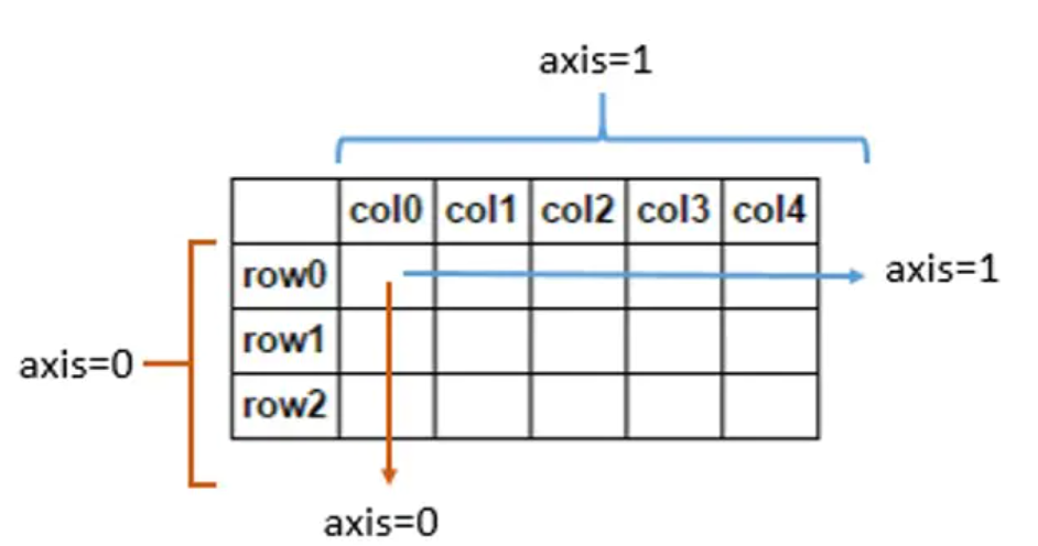
axis
“axis=0表示跨行,axis=1表示跨列,作为方法动作的副词”
squeeze()函数
函数原型:numpy.squeeze(a, axis=None)
函数功能:把数组中shape中为1的维度去掉。默认删除a数组中所有shape中为1的维度,axis指定要删除的维度,axis=0表示第0维,若是该维度的shape不为1,则会报错。
a = [ [[1,2]], [[3,4]] ]    # shape为2*1*2
# 删除中间为1的维度后
a = [ [1,2], [3,4] ]  # 看起来就像是将“穿”的夹层多余的衣服(括号)脱掉一层
我们会在PyTorch中使用使用squeeze()和unsqueeze()进行降维和升维的步骤。
unsqueeze()函数的功能是在tensor的某个维度上添加一个维数为1的维度,这个功能用view()函数也可以实现。这一功能尤其在神经网络输入单个样本时很有用,由于pytorch神经网络要求的输入都是mini-batch型的,维度为[batch_size, channels, w, h],而一个样本的维度为[c, w, h],此时用unsqueeze()增加一个维度变为[1, c, w, h]就很方便了。
median()
edian(a,
axis=None,
out=None,
overwrite_input=False,
keepdims=False)a:输入的数组;
axis:计算哪个轴上的均值,比如输入是二维数组,那么axis=0对应行,axis=1对应列;
out:用于放置求取中位数后的数组。 它必须具有与预期输出相同的形状和缓冲区长度;
**overwrite_input :**一个bool型的参数,默认为Flase。如果为True那么将直接在数组内存中计算,这意味着计算之后原数组没办法保存,但是好处在于节省内存资源,Flase则相反;
keepdims:一个bool型的参数,默认为Flase。如果为True那么求取中位数的那个轴将保留在结果中;
计算沿指定轴的均值,返回数组元素的均值
>>> a = np.array([[10, 7, 4], [3, 2, 1]])
>>> a
array([[10,  7,  4],
       [ 3,  2,  1]])
>>> np.median(a)
3.5
>>> np.median(a, axis=0)
array([ 6.5,  4.5,  2.5])
>>> np.median(a, axis=1)
array([ 7.,  2.])
>>> m = np.median(a, axis=0)
>>> out = np.zeros_like(m)
>>> np.median(a, axis=0, out=m)
array([ 6.5,  4.5,  2.5])
>>> m
array([ 6.5,  4.5,  2.5])
>>> b = a.copy()
>>> np.median(b, axis=1, overwrite_input=True)
array([ 7.,  2.])
>>> assert not np.all(a==b)
>>> b = a.copy()
>>> np.median(b, axis=None, overwrite_input=True)
3.5
expand_dims()
这个东西的主要作用,就是增加一个维度。
现在我们假设有一个数组A,数组A是一个两行三列的矩阵。大小我们记成(2,3)。
先明白一个常识,计算机中计数,一般是从0开始的。
所以(2,3)这个两行三列的矩阵,
它的第“0”维,就是这个“2”行;第“1”维,就是这个“3”列。
这个函数的作用,就是在第“axis”维,加一个维度出来,原先的“维”,推到右边去。
比如我们设置axis为0,那[A矩阵]的大小就变成了(1,2,3),就从2*3的二维矩阵变成了一个1*2*3的三维矩阵。如果设置[axis]为1,矩阵大小就变成了(2,1,3),变成了一个2*1*3的三维矩阵。axis为2的时候,就变成(2,3,1)啦。
那么,说了这么多,矩阵的形式变了,那么矩阵里面的数字怎么变的呢?
举个例子:
假设现在矩阵是2*3的矩阵,六个数字
1 2 3
4 5 6
初中和高中所学的平面直角坐标系和空间直角坐标系还记得吗?
我们设置axis为0,矩阵从2*3的二维矩阵变成了1*2*3的三维矩阵。
我们假设原来是一个二维平面,横坐标为x,纵坐标为y, 2*3的矩阵在这个XOY平面上。此时就是一个二维矩阵,(根本就没有z轴)
而变换以后,现在变成了三维矩阵,变成了一个空间直角坐标系,,有x,y,z三个轴。
原先的2*3的矩阵从XOY平面移动到了YOZ平面
(我们把原先的矩阵当成一个平摊在桌面上的纸片,变换以后,相当于给它立起来了),然后原先的X轴的“厚度”为1,此时虽然形式还是原来的数字,但是多了一个轴。
那如果设置axis为1呢?
就是从XOY面的矩阵,给它立起来到XOZ平面,在Y轴的厚度为1。
设置axis为2,就是从XOY面的矩阵,还是放在XOY面上。但是这时候多了一个z轴,(相当于这个操作之后可以在桌面的纸片上面,叠加新的纸片了)
——————————————————————————————————
这时候我们再看矩阵
1 2 3
4 5 6
原先A[0][0]对应1,A[0][1]对应2,A[0][2]对应3,A[1][0]对应4……
如果设置axis为0,这时候矩阵从XOY平面移动到了YOZ平面,X轴只有一个值
那么,变换后的矩阵A’的第一个维度,只有一个值,就只能是0
A’[0][0][0]是1,A[0][0][1]是2,A[0][0][2]是3
A’[0][1][0]是4,A[0][1][1]是5,A[0][1][2]是6
A’[0][0]不指定第三维,那么就是[1,2,3]
A’[0][1]不指定第三维,就是[4,5,6]
那A[1][0][0]……呢?不好意思,没有,因为第一维只能取一个数,就是0。
axis为1,2都同理。
可能说的有点啰嗦了。
如果是三维矩阵变成四维矩阵,那就不好直接想象样子了。但是道理是一样的。
a = np.array([122,34,45])
b = np.expand_dims(a,0)
print(b)
'''
[[122  34  45]]
'''
b = np.expand_dims(a,1)
print(b)
'''
[[122]
 [ 34]
 [ 45]]
'''
b = np.expand_dims(a,-1)
print(b)
'''
[[122]
 [ 34]
 [ 45]
'''
random
seed()
可以通过输入int或arrat_like来使得随机的结果固定;使实验可重复,对于同一个seed,生成的随机数相同
numpy.random.seed(seed=None) random()
生成指定维度的[0,1)间的随机数
e = np.random.random((2,2)) # Create an array filled with random values
print(e)
'''
[[0.44790028 0.50508009]
 [0.99214661 0.3657341 ]]
'''
random_sample()
用于在numpy中进行随机采样的函数之一。它返回指定形状的数组,并在半开间隔中将其填充为随机浮点数[0.0, 1.0).
用法: numpy.random.random_sample(size=None)rand(d0,d1...dn)
通过本函数可以返回一个或一组服从“0~1”均匀分布的随机样本值。随机样本取值范围是[0,1),不包括1。 应用:在深度学习的Dropout正则化方法中,可以用于生成dropout随机向量(dl),例如(keep_prob表示保留神经元的比例):
dl = np.random.rand(al.shape[0],al.shape[1]) < keep_prob
np.random.rand(4,3)out:
array([[0.27388623, 0.26940718, 0.13914399],
[0.79281929, 0.82086991, 0.18488757],
[0.09359689, 0.08408097, 0.36463413],
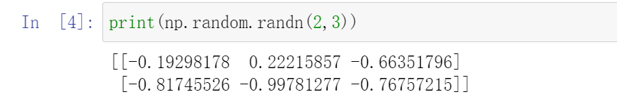
[0.02924776, 0.81743324, 0.26361082]])randn()
randn函数返回一个或一组样本,具有[标准正态分布]。
numpy.random.randint(low, high=None, size=None, dtype=’l’)
- 从区间[low,high)返回随机整数
- 参数:low为最小值,high为最大值,size为数组维度大小,dtype为数据类型,默认的数据类型是np.int
- high没有填写时,默认生成随机数的范围是[0,low)
np.random.normal(mu, sigma, size)
随机生成服从正太分布的随机数。
$\mu$为均值
$\sigma$为标准差
$size$: int or tuple of ints, optional。输出形状。如果给定的形状是,例如,(m, n, k),那么将绘制m x n x k的样本。默认为无,在这种情况下,将返回一个单一的值。
# coding=utf-8
'''
作者:采石工
来源:知乎
'''
import numpy as np
from numpy.linalg import cholesky
import matplotlib.pyplot as plt
sampleNo = 1000;
# 一维正态分布
# 下面三种方式是等效的
mu = 3
sigma = 0.1
np.random.seed(0)
s = np.random.normal(mu, sigma, sampleNo )
plt.subplot(141)
plt.hist(s, 30, normed=True)
np.random.seed(0)
s = sigma * np.random.randn(sampleNo ) + mu
plt.subplot(142)
plt.hist(s, 30, normed=True)
np.random.seed(0)
s = sigma * np.random.standard_normal(sampleNo ) + mu
plt.subplot(143)
plt.hist(s, 30, normed=True)
# 二维正态分布
mu = np.array([[1, 5]])
Sigma = np.array([[1, 0.5], [1.5, 3]])
R = cholesky(Sigma)
s = np.dot(np.random.randn(sampleNo, 2), R) + mu
plt.subplot(144)
# 注意绘制的是散点图,而不是直方图
plt.plot(s[:,0],s[:,1],'+')
plt.show()
choice(a, size=None, replace=True, p=None)
- 从给定的一位数组中生成一个随机样本
- a要求输入一维数组类似数据或者是一个int;size是生成的数组纬度,要求数字或元组;replace为布尔型,决定样本是否有替换;p为样本出现概率
///p是一个list,p的size 必须与a的size一致,p中每个元素对应了a中每个元素被选择的概率
np.random.choice(list_tmp,size = (3,3),p = [0.1,0.6,0.1,0.1,0.1])
shuffle(x)
现场修改序列,改变自身内容。(类似洗牌,打乱顺序)
>>> arr = np.arange(10)
>>> np.random.shuffle(arr)
>>> arr
[1 7 5 2 9 4 3 6 0 8]
default_rng(myseed)
打乱数据
myseed = 42069
rng = np.random.default_rng(myseed)
df = pandas.read_csv('iris.csv')
data = np.array(df)
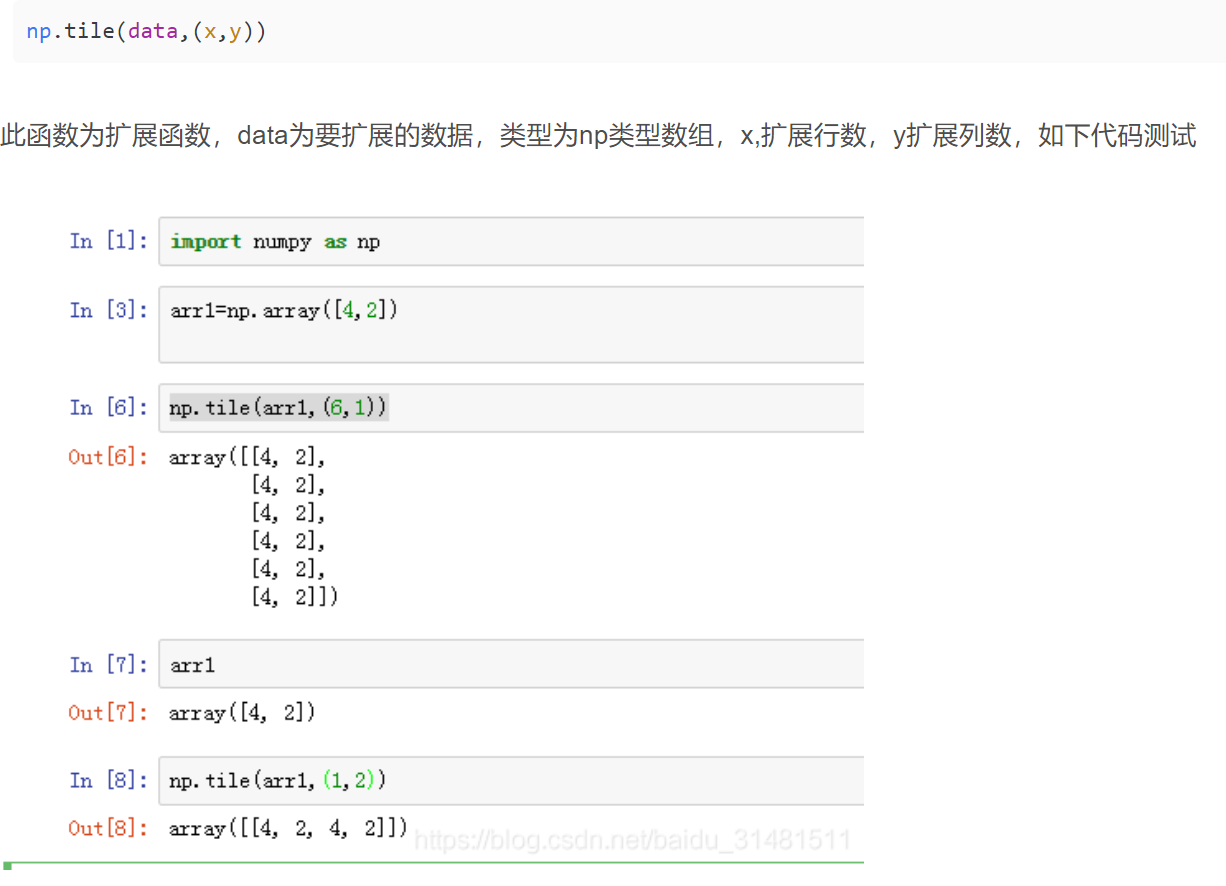
rng.shuffle(data)tile()
std()
计算标准差
因此,想要正确调用,必须使ddof=1:
ddof : int, optional
Means Delta Degrees of Freedom. The divisor used in calculations is N - ddof, where N represents the number of elements. By default ddof is zero.
>>> np.std([1,2,3], ddof=1)
1.0
广播(broadcasting)
在Numpy中,如果参与运算的两个数组或者矩阵的形状不同,则解释器将双方的各个维数右对齐,并开始从右至左依次比较对应的两个维数是否相等。如果只存在“相等“、”不相等但有一方为1“,”有一方没有对应的维数“这三种情况,则进行广播,否则报错。
例如,一方的维数为6x3x5,另一方的维数是3x1,则进行广播,运算的结果为一个6x3x5大小的数组。再例如,一方为行向量,维数为1xm,另一方为标量b,维数为1x1,则进行广播,广播的结果是将标量b拉伸为与前一方形状相同的1xm维行向量,其中的元素都是标量b的副本,然后再进行运算。
np.power(x1,x2)
x1和x2可以是整数类型或数组或者array类型。
x1 = np.array([[0,1],[2,3]])
x2 = np.array([[3,4],[4,5]])
result = np.power(x1,x2) # 实际就是相应位置的前者的后者次方(x1[i,j]**x2[i,j])

#输出
'''
[[  0   1]
 [ 16 243]]
'''
numpy.where–将条件逻辑表述为数组运算
result = np.where(cond, xarr, yarr)np.where的第二个和第三个参数不必是数组,它们都可以是标量值。在数据分析工作中,where通常用于根据另一个数组而产生一个新的数组。假设有一个由随机数据组成的矩阵,你希望将所有正值替换为2,将所有负值替换为-2。若利用np.where,则会非常简单:
In [172]: arr = np.random.randn(4, 4)

In [173]: arr
Out[173]:
array([[-0.5031, -0.6223, -0.9212, -0.7262],
       [ 0.2229,  0.0513, -1.1577,  0.8167],
       [ 0.4336,  1.0107,  1.8249, -0.9975],
       [ 0.8506, -0.1316,  0.9124,  0.1882]])

In [174]: arr > 0
Out[174]:
array([[False, False, False, False],
       [ True,  True, False,  True],
       [ True,  True,  True, False],
       [ True, False,  True,  True]], dtype=bool)

In [175]: np.where(arr > 0, 2, -2)
Out[175]:
array([[-2, -2, -2, -2],
       [ 2,  2, -2,  2],
       [ 2,  2,  2, -2],
       [ 2, -2,  2,  2]])
使用np.where,可以将标量和数组结合起来。例如,我可用常数2替换arr中所有正的值:
In [176]: np.where(arr > 0, 2, arr) # set only positive values to 2
Out[176]:
array([[-0.5031, -0.6223, -0.9212, -0.7262],
[ 2. , 2. , -1.1577, 2. ],
[ 2. , 2. , 2. , -0.9975],
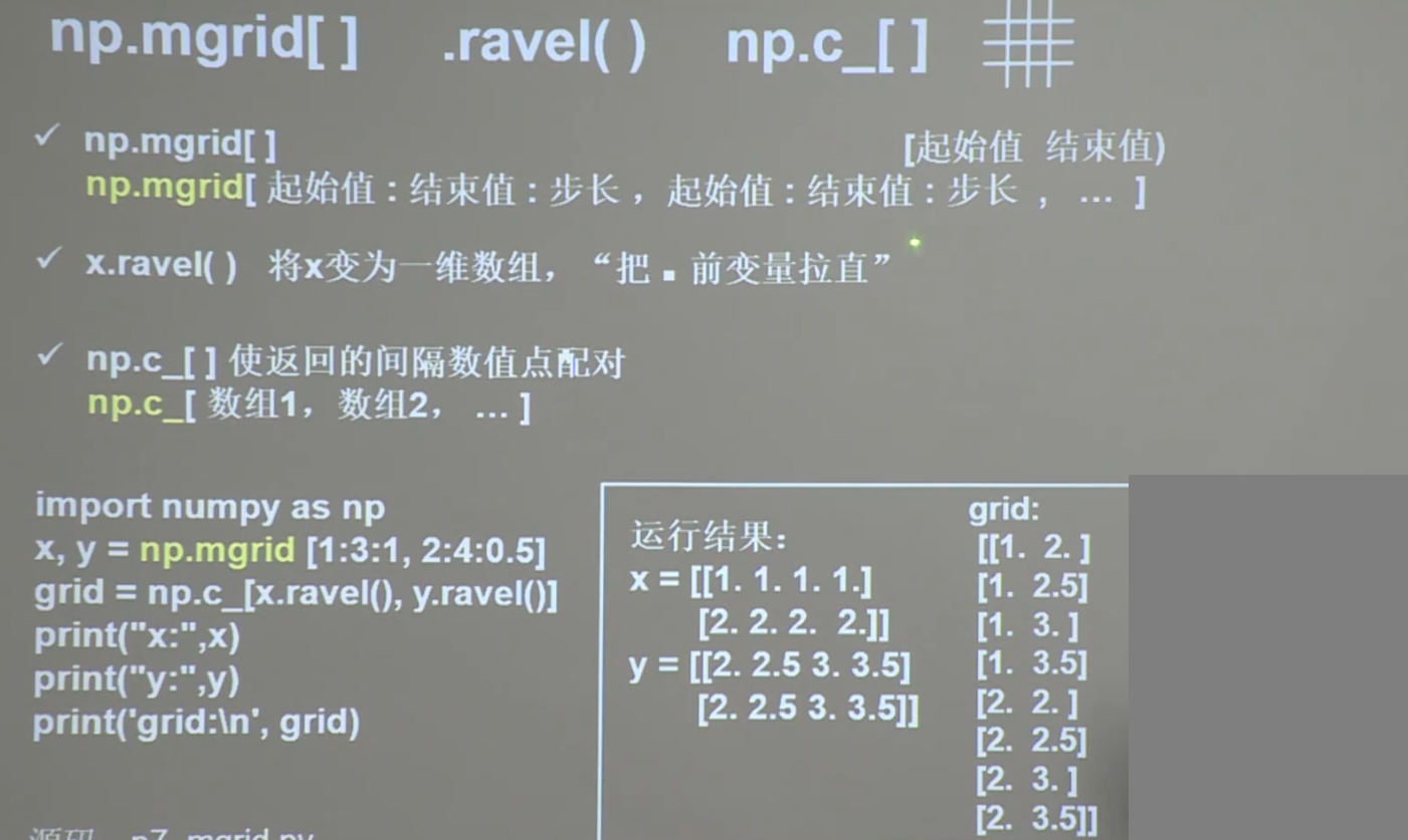
[ 2. , -0.1316, 2. , 2. ]])np.mgrid[] np.ravel np.c_[]
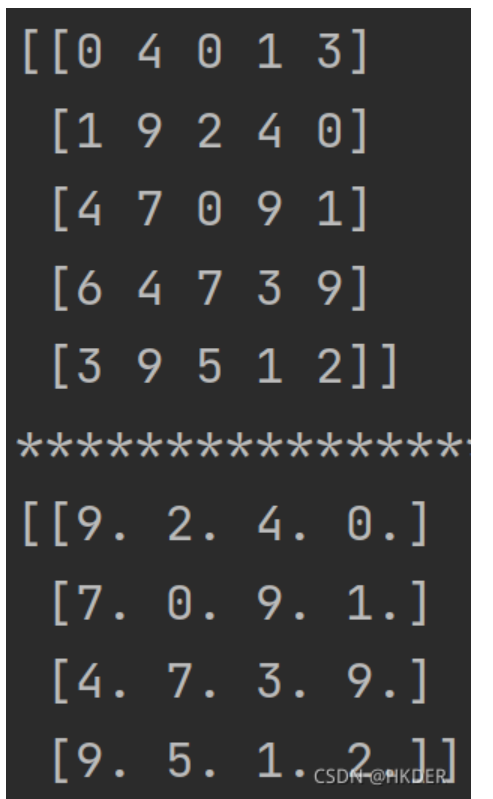
数据数组去除第一行和第一列data = np.array(data[1:])[:, 1:]
import numpy as np
data = np.random.randint(0,10,(5,5))
print(data)
print('*******************************')
data1 = np.array(data[1:])[:, 1:].astype(float)
print(data1)
结果:
np.fromstring
if __name__ == "__main__":
    TARGET_PHRASE = 'You get it!'
    TARGET_ASCII = np.fromstring(TARGET_PHRASE, dtype=np.uint8)  # convert string to number
    print(TARGET_PHRASE,TARGET_ASCII)
    print(len(TARGET_PHRASE),TARGET_ASCII.shape)

'''
You get it! [ 89 111 117  32 103 101 116  32 105 116  33]
11 (11,)
'''不过这个方法现在已经过时了,现在常用numpy.frombuffer
if __name__ == "__main__":
TARGET_PHRASE = 'You get it!' # target DNA
TARGET_ASCII = np.frombuffer(TARGET_PHRASE.encode() ,dtype=np.uint8) # convert string to number
print(TARGET_PHRASE,TARGET_ASCII)
print(len(TARGET_PHRASE),TARGET_ASCII.shape)
s = TARGET_ASCII.tobytes() .decode('ascii')
print(s)
'''
You get it! [ 89 111 117 32 103 101 116 32 105 116 33]
11 (11,)
You get it!
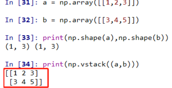
'''np.vstack()
按垂直方向(行顺序)堆叠数组构成一个新的数组
堆叠的数组需要具有相同的维度
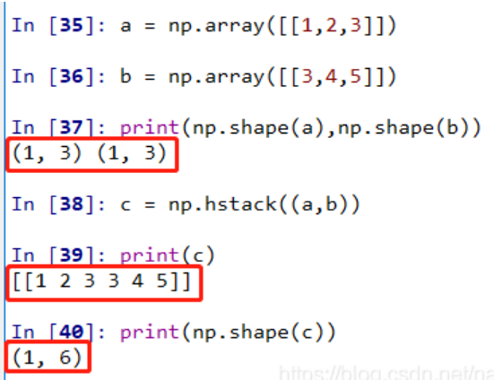
np.hstack()
按水平方向(列顺序)堆叠数组构成一个新的数组
堆叠的数组需要具有相同的维度
matplotlib
小技巧:
Jupyter Notebook 上面用 Matplotlib 了,但是不知道大家看到画出来那一坨糊糊的东西会不会跟我一样浑身难受。实际上,只要多加一行配置,就能够让 Matplotlib 在 Jupyter Notebook 上面输出矢量图了:
import matplotlib
import matplotlib.pyplot as plt
%matplotlib inline
%config InlineBackend.figure_format = 'svg'
savefig 只要指定文件名后缀是 .pdf 或者 .eps 就能生成能方便地插入 latex 的图片了!
plt.savefig('tmp.pdf', bbox_inches='tight')
plt.show()
matplotlib实用函数
def use_svg_display():
    """使用svg格式在Jupyter中显示绘图"""
    backend_inline.set_matplotlib_formats('svg')

def set_figsize(figsize=(3.5, 2.5)):
    """设置matplotlib的图表大小"""
    use_svg_display()
    d2l.plt.rcParams['figure.figsize'] = figsize

def set_axes(axes, xlabel, ylabel, xlim, ylim, xscale, yscale, legend):
    """设置matplotlib的轴"""
    axes.set_xlabel(xlabel)
    axes.set_ylabel(ylabel)
    axes.set_xscale(xscale)
    axes.set_yscale(yscale)
    axes.set_xlim(xlim)
    axes.set_ylim(ylim)
    if legend:
        axes.legend(legend)
    axes.grid()

def plot(X, Y=None, xlabel=None, ylabel=None, legend=None, xlim=None,
         ylim=None, xscale='linear', yscale='linear',
         fmts=('-', 'm--', 'g-.', 'r:'), figsize=(3.5, 2.5), axes=None):
    """绘制数据点"""
    if legend is None:
        legend = []

    set_figsize(figsize)
    axes = axes if axes else d2l.plt.gca()

    def has_one_axis(X):
        return (hasattr(X, "ndim") and X.ndim == 1 or isinstance(X, list)
                and not hasattr(X[0], "__len__"))

    if has_one_axis(X):
        X = [X]
    if Y is None:
        X, Y = [[]] * len(X), X
    elif has_one_axis(Y):
        Y = [Y]
    if len(X) != len(Y):
        X = X * len(Y)
    axes.cla()
    for x, y, fmt in zip(X, Y, fmts):
        if len(x):
            axes.plot(x, y, fmt)
        else:
            axes.plot(y, fmt)
    set_axes(axes, xlabel, ylabel, xlim, ylim, xscale, yscale, legend)
使用上述函数画图
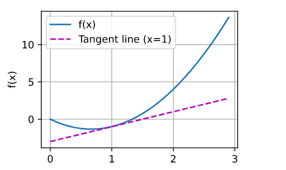
eg.1
def f(x):
    return 3 * x ** 2 - 4 * x
x = np.arange(0, 3, 0.1)
plot(x, [f(x), 2 * x - 3], 'x', 'f(x)', legend=['f(x)', 'Tangent line (x=1)'])
eg.2
x = torch.arange(-8.0, 8.0, 0.1, requires_grad=True)
y = torch.relu(x)
d2l.plot(x.detach(), y.detach(), 'x', 'relu(x)', figsize=(5, 2.5))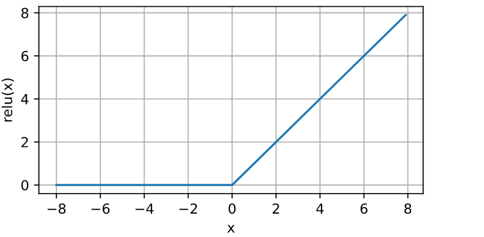
import numpy as np
import matplotlib.pyplot as plt
from pylab import xticks,yticks,np

yticks(np.linspace(0,1.,11,endpoint=True))
plt.xlabel("epoch")  # x的轴标签
plt.ylabel("accuracy")  # y的轴标签
plt.legend(["准确率"])  # 图例名称
plt.title("The Image Of Multinomial Logistic Regression")# 图像名称
plt.show()
plt.plot()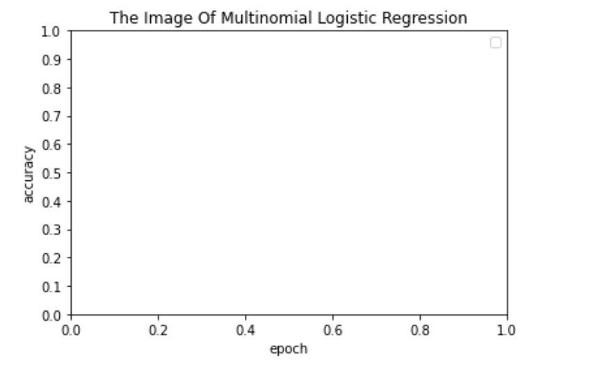
绘制两条简单的曲线
import numpy as np
import matplotlib.pyplot as plt

x = np.arange(0, 3 * np.pi, 0.1)
y_sin = np.sin(x)
y_cos = np.cos(x)

# Plot the points using matplotlib
plt.plot(x, y_sin)
plt.plot(x, y_cos)
plt.xlabel('x axis label')
plt.ylabel('y axis label')
plt.title('Sine and Cosine')
plt.legend(['Sine', 'Cosine'])

# 自定义刻度
#x_list = [i for i in range(-10,11)]
#plt.xticks(x_list)

plt.show()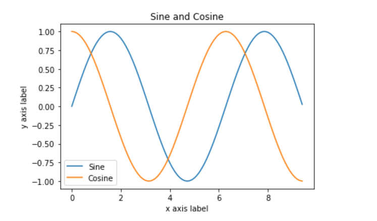
绘制 $f(x)=3 x^2+7x-9$的图像
import numpy as np
import matplotlib.pyplot as plt

x = np.linspace(0, 8)  # x取值范围
y = 3 * x ** 2 + 7 * x - 9  # y函数
plt.plot(x, y, )  # 以x为取值范围标定横坐标,y为纵坐标
plt.rcParams['font.sans-serif'] = ['SimHei']  # 解析中文字体
plt.xlabel("x的取值")  # x的轴标签
plt.ylabel("y的值")  # y的轴标签
plt.text(7, 100, "我是曲线")  # 曲线名称(标定位置)
plt.legend(["我是图例"])  # 图例名称
plt.title("the image of function")# 图像名称
plt.show()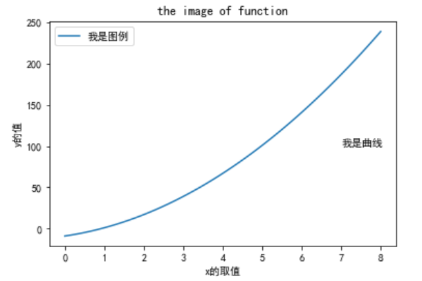
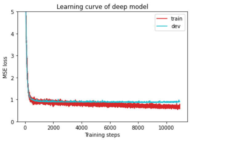
绘制学习曲线
def plot_learning_curve(loss_record, title=''):
    ''' Plot learning curve of your DNN (train & dev loss) '''
    total_steps = len(loss_record['train'])
    x_1 = range(total_steps) # train曲线 x点集范围
    x_2 = x_1[::len(loss_record['train']) // len(loss_record['dev'])] # dev曲线 x点集范围
    figure(figsize=(6, 4)) # 图像大小
    plt.plot(x_1, loss_record['train'], c='tab:red', label='train') # 绘制train曲线
    plt.plot(x_2, loss_record['dev'], c='tab:cyan', label='dev')# 绘制dev曲线
    plt.ylim(0.0, 5.) # 限制 y轴取值范围
    plt.xlabel('Training steps')# x轴名称
    plt.ylabel('MSE loss')# y轴名称
    plt.title('Learning curve of {}'.format(title))# 图标题
    plt.legend()
    plt.show()
绘制预测曲线拟合程度
def plot_pred(dv_set, model, device, lim=35., preds=None, targets=None):
    ''' Plot prediction of your DNN '''

    if preds is None or targets is None: # test
        model.eval()
        preds, targets = [], []
        for x, y in dv_set:
            x, y = x.to(device), y.to(device)
            with torch.no_grad():
                pred = model(x)
                preds.append(pred.detach().cpu())
                targets.append(y.detach().cpu())
        preds = torch.cat(preds, dim=0).numpy()
        targets = torch.cat(targets, dim=0).numpy()

    figure(figsize=(5, 5))
    plt.scatter(targets, preds, c='r', alpha=0.5)# 绘制点图
    plt.plot([-0.2, lim], [-0.2, lim], c='b')
    plt.xlim(-0.2, lim)
    plt.ylim(-0.2, lim)
    plt.xlabel('ground truth value')
    plt.ylabel('predicted value')
    plt.title('Ground Truth v.s. Prediction')
    plt.show()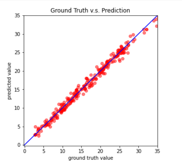
绘制点以及曲线
colors = []
for i in y:
    t = i.item(0)
    if t > 0:
        colors.append('red')
    else:
        colors.append('blue')
plt.scatter(x,y,c=colors)
x_range = np.linspace(0,80)
plt.ylim(-5.,3.0)
plt.plot(x_range,(w*x_range+b).T.squeeze()) 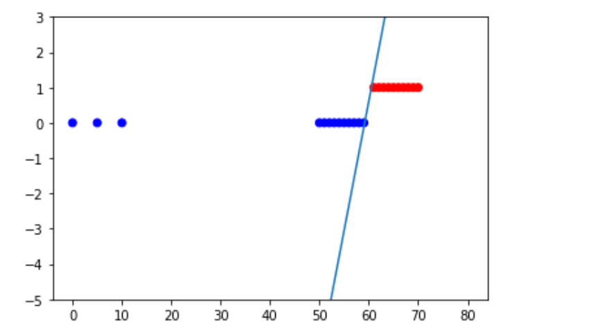
子图绘制
方式1
fig = plt.figure()
ax1 = fig.add_subplot(2, 2, 1)
ax2 = fig.add_subplot(2, 2, 2)
ax3 = fig.add_subplot(2, 2, 3)

ax1.hist(np.random.randn(100), bins=20, color='k', alpha=0.3)
ax2.scatter(np.arange(30), np.arange(30) + 3 * np.random.randn(30))

x = np.linspace(-10,10,100,dtype=float)
ax3.plot(x,np.sin(x))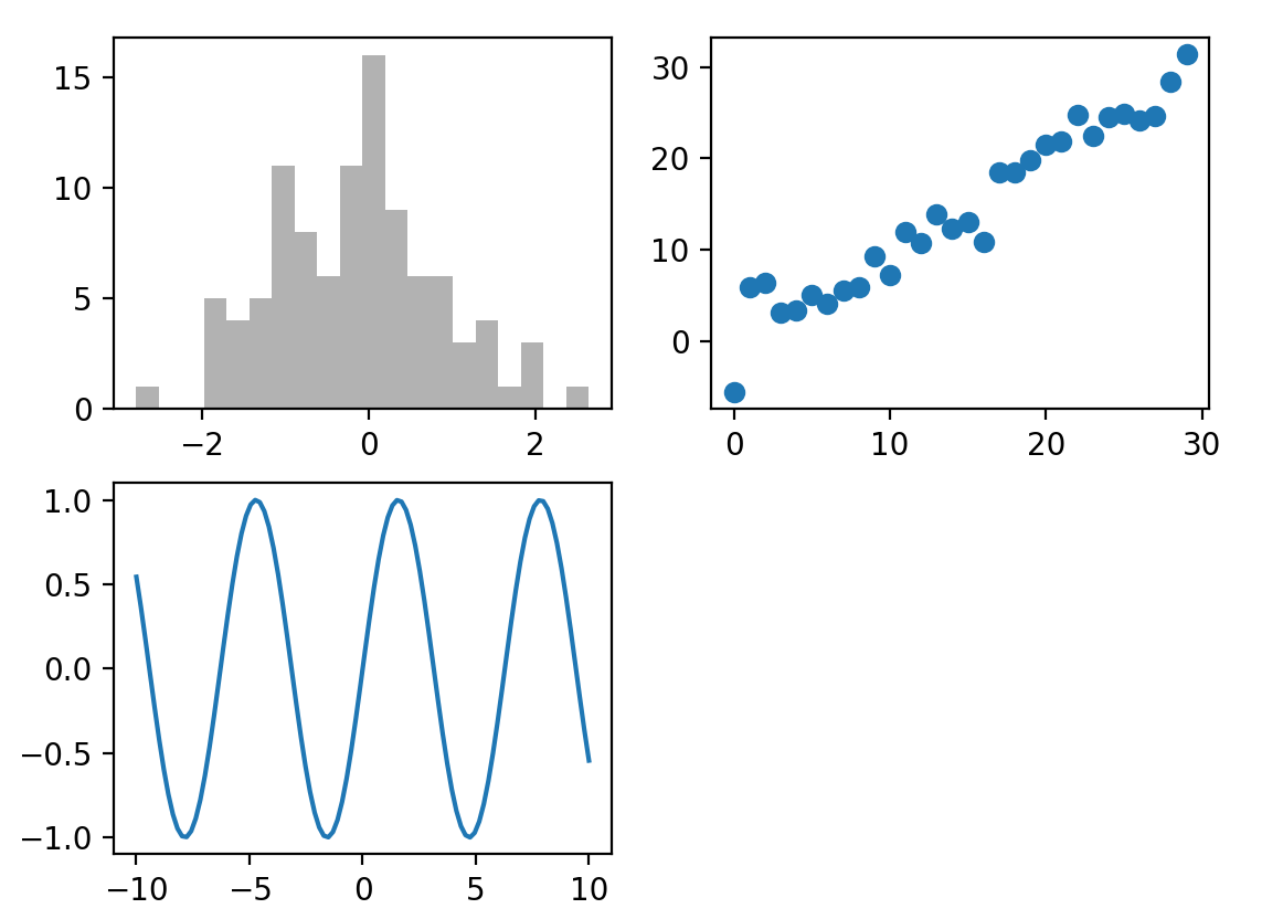
方式2
x = np.arange(0, 3 * np.pi, 0.1)
y_sin = np.sin(x)
y_cos = np.cos(x)

# Set up a subplot grid that has height 2 and width 1,
# and set the first such subplot as active.
plt.subplot(2, 1, 1)

# Make the first plot
plt.plot(x, y_sin)
plt.title('Sine')

# Set the second subplot as active, and make the second plot.
plt.subplot(2, 1, 2)
plt.plot(x, y_cos)
plt.title('Cosine')

# Show the figure.
plt.show()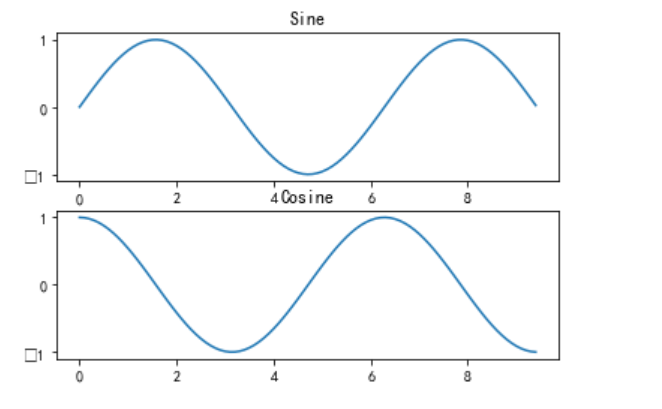
%matplotlib inline是IPython的魔法命令之一,用于在IPython notebook或Jupyter notebook中显示图形输出。具体而言,它会将matplotlib生成的图形嵌入到notebook中,并且不需要在单独的窗口中打开它们。
当在notebook中执行matplotlib绘图代码时,如果没有使用%matplotlib inline命令,则matplotlib默认情况下会创建一个新的窗口来显示图形。而使用%matplotlib inline命令后,所有的图形输出将直接显示在notebook中,便于查看和分析。
需要注意的是,%matplotlib inline命令必须在导入matplotlib库之前执行,才能确保所有的图形都能被正确地显示在notebook中。
利用matplotlib进行动态绘制(连续图像绘制)
因为python可视化库matplotlib的显示模式默认为阻塞(block)模式(即:在plt.show()之后,程序会暂停到那儿,并不会继续执行下去)。如何展示动态图或多个窗口 呢?使用plt.ion()这个函数,使matplotlib的显示模式转换为交互(interactive)模式。即使在脚本中遇到plt.show( ),代码还是会继续执行。在plt.show()之前一定不要忘了加plt.ioff(),如果不加,界面会一闪而过,并不会停留。
在阻塞模式下:
1、打开一个窗口以后必须关掉才能打开下一个新的窗口。这种情况下,默认是不能像Matlab一样同时开很多窗口进行对比的。
2、plt.plot(x)或plt.imshow(x)是直接出图像,需要plt.show()后才能显示图像。
在交互模式下:
1、plt.plot(x)或plt.imshow(x)是直接出图像,不需要plt.show()。
2、如果在脚本中使用ion()命令开启了交互模式,没有使用ioff()关闭的话,则图像会一闪而过,并不会常留。要想防止这种情况,需要在plt.show()之前加上ioff()命令。
import matplotlib.pyplot as plt
if __name__ == "__main__":
    plt.ion()  # 打开交互模式
    # 同时打开两个窗口显示图片
    x = np.linspace(-10,10,100)
    y = np.sin(x)
    plt.plot(x,y)
    for i in range(4):
        if 'sca' in globals(): sca.remove()
        sca = plt.scatter([i,i+1], [0.5,0.5], s=200, lw=0, c='red', alpha=0.5);
        plt.pause(0.05)
    plt.ioff()
    plt.show()
tensorflow
tensor创建
tf.zeros(维度)
创建全为0的tensor
tf.ones(维度)
创建全为1的tensor
tf.fill(维度,指定值)
创建指定值的tensor
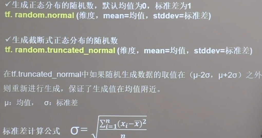
tf.random.normal(维度,mean=均值,stddev=标准差)
生成正态分布的随机数,默认均值为0,标准差为1
tf.random.truncated_normal(维度,mean=均值,stddev=标准差)
保证生成的随机数在$\mu$+/-$2\sigma$之内,数据更加向均值集中
tf.random.uniform(维度,minval=最小值,maxval=最大值)
生成均匀分布随机数[minval,maxval)
常用函数
tf.cast(张量名,dtype=数据类型)
强制tensor转换为该数据类型
tf.reduce_min(张量名)
计算张量维度上元素最小值
tf.reduce_max(张量名)
计算张量维度上的最大值
tf.reduce_mean(张量名,axis=)
计算张量沿着指定维度的平均值
tf.reduce_sum(张量名,axis=)
计算张量沿着指定维度的和
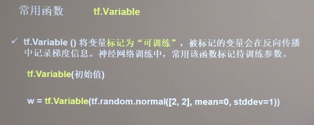
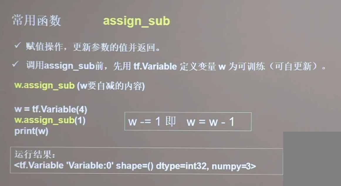
tf.Variable()
将变量标记为可训练的
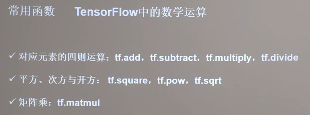
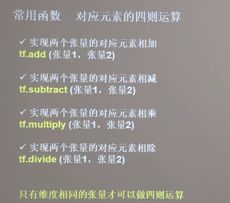
tf中常用的数学运算
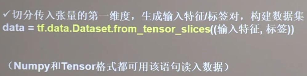
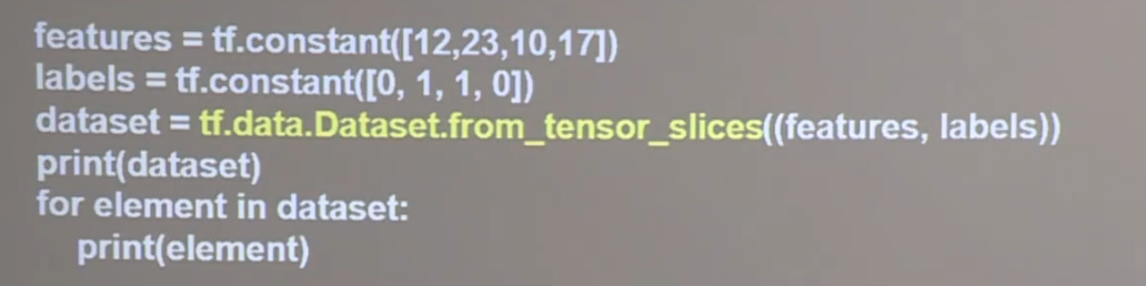
tf.data.Dataset.from_tensor_slices
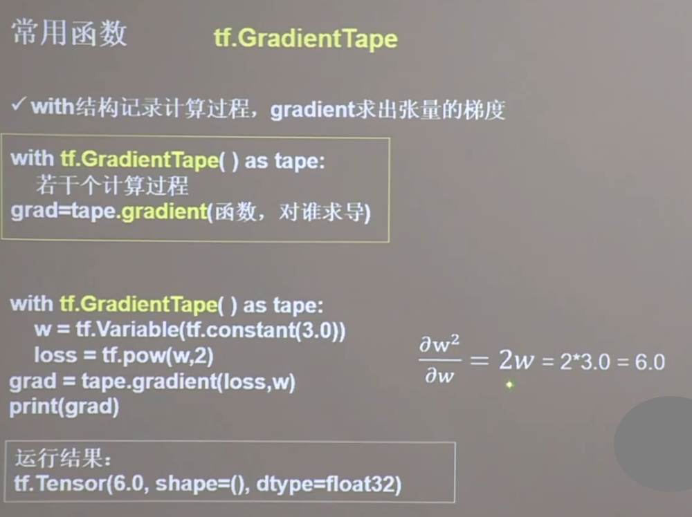
tf.GradientTape
with结构中记录计算过程,gradient求出张量的梯度
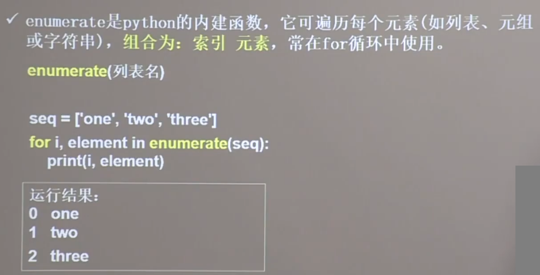
enumerate
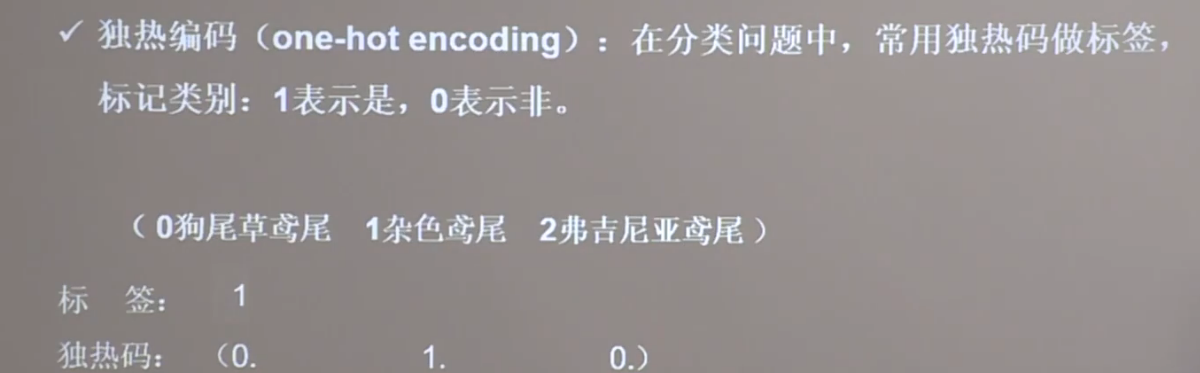
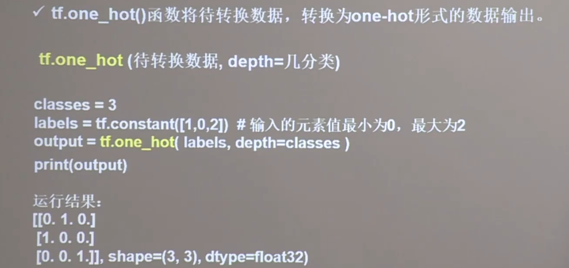
tf.one_hot
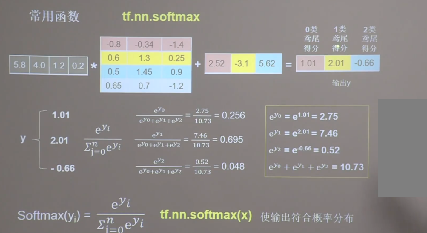
tf.nn.softmax
assign_sub
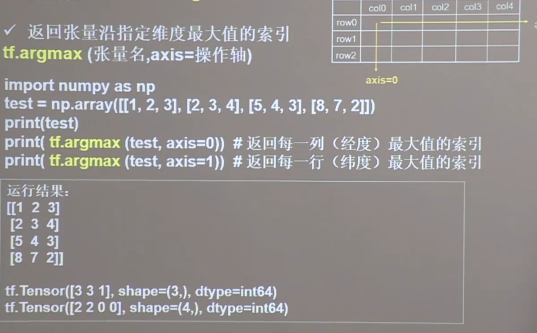
tf.argmax
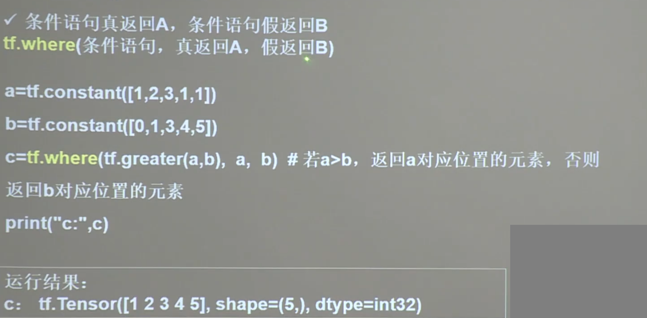
tf.where
tf.distributions.Normal(self.mu, self.sigma)
根据Mu和sigma求出一个正太分布,这个是随机的正态分布
tf.clip_by_value
tf.clip_by_value(A, min, max):输入一个张量A,把A中的每一个元素的值都压缩在min和max之间。小于min的让它等于min,大于max的元素的值等于max。
tensorflow_probability
tensorflow_probability 是基于 TensorFlow 的一个概率编程库,它提供了许多用于概率建模和推断的工具和算法,可以用于深度学习、统计学习、贝叶斯推断、概率编程等领域。它是 TensorFlow 生态系统中的一个子项目,由 TensorFlow 官方支持和维护。
tensorflow_probability 包含了很多常用的概率分布类,例如正态分布、多项式分布、贝塔分布等,还包括许多概率模型,例如高斯混合模型、马尔可夫链蒙特卡罗(MCMC)模型等。此外,它还提供了许多常用的推断算法,例如变分推断、哈密顿蒙特卡罗(HMC)算法等,可以用于学习和推断概率模型。
tensorflow_probability 的设计理念是利用 TensorFlow 的计算图和自动微分机制,为概率编程提供高效、可扩展和易用的工具。因此,它与 TensorFlow 紧密集成,可以直接利用 TensorFlow 的张量操作和优化器等功能,实现高效的概率编程。
tfp.distributions.MultivariateNormalFullCovariance
MultivariateNormalFullCovariance 是 TensorFlow 中的一个概率分布类,表示一个具有多元正态分布的随机变量。它接受两个参数:均值向量和协方差矩阵,可以使用它来构建一个多元正态分布的概率模型。
下面是一个示例代码,展示了如何使用 MultivariateNormalFullCovariance 类:
import tensorflow_probability as tfp
import tensorflow as tf

# 定义均值向量和协方差矩阵
mu = [0., 1.]
cov = [[1., 0.5], [0.5, 2.]]

# 创建一个多元正态分布模型
mvn = tfp.distributions.MultivariateNormalFullCovariance(loc=mu, covariance_matrix=cov)

# 生成一些样本
samples = mvn.sample(10)

# 计算概率密度函数
pdf = mvn.prob(samples)

print("samples: \n", samples)
print("pdf: \n", pdf)

'''
samples:
 tf.Tensor(
[[-0.76739496  2.204533  ]
 [-0.5291017  -1.2480607 ]
 [ 0.2066121  -0.3552009 ]
 [-0.3798596   2.0005732 ]
 [-0.3424486   1.2140272 ]
 [-0.9631925   1.9374372 ]
 [-0.343555    1.0946357 ]
 [ 0.83072865 -0.9090407 ]
 [ 0.22511458 -0.35162723]
 [-1.363401    1.9629669 ]], shape=(10, 2), dtype=float32)
pdf:
 tf.Tensor(
[0.04359382 0.03398798 0.06413195 0.07466278 0.1087476  0.04255811
 0.11113843 0.01819854 0.06357419 0.02192882], shape=(10,), dtype=float32)
'''
在上面的代码中,我们首先定义了均值向量 mu 和协方差矩阵 cov。然后,我们使用这些参数创建了一个 MultivariateNormalFullCovariance 对象 mvn,它表示一个多元正态分布。接着,我们使用 mvn.sample(10) 生成了 10 个样本,并计算了这些样本的概率密度函数。
你可以根据自己的需求来修改均值向量和协方差矩阵,从而创建不同的多元正态分布模型。另外,MultivariateNormalFullCovariance 类还提供了其他一些方法,例如 log_prob()、entropy() 等,可以用于计算概率密度函数的对数、熵等。
在上面的例子中,prob 函数是 tensorflow_probability 中 MultivariateNormalFullCovariance 类的一个方法,它的作用是计算给定样本的概率密度函数值。
具体来说,prob 方法接受一个张量作为输入,这个张量的每一行代表一个样本,每一列代表一个特征。它返回一个形状与输入张量相同的张量,每个元素代表相应样本的概率密度函数值。
在本例中,我们首先通过 mvn.sample(10) 生成了 10 个样本,然后通过 mvn.prob(samples) 计算了这些样本的概率密度函数值。这个结果告诉我们这些样本在多元正态分布模型下的概率密度大小,可以用于评估样本的合理性、寻找异常值等任务。
需要注意的是,prob 方法仅适用于概率密度函数已知的分布,对于一些无法计算概率密度函数的分布,例如混合分布,需要使用其他方法来评估样本的合理性,例如计算似然函数、负对数似然函数等。
需要注意的是,prob 方法返回的值并不是概率,而是概率密度函数的值。
在概率论中,概率密度函数(Probability Density Function,简称 PDF)是指某个随机变量落在某个区间内的概率在该区间长度趋于零时的极限,即密度函数在该点处的函数值。因此,概率密度函数的值并不代表概率,而是代表了某个区间内的概率密度大小。
对于连续型随机变量,我们无法像离散型随机变量那样直接计算概率,而是需要通过概率密度函数进行计算。具体来说,某个区间内的概率可以通过该区间内概率密度函数的积分来计算。
在本例中,mvn.prob(samples) 返回的是样本在多元正态分布模型下的概率密度函数值,它的大小反映了该样本在该分布下的密度大小,而不是该样本出现的概率。因此,在实际使用中需要注意区分概率和概率密度函数的概念。
sklearn
sklearn流水线(Pipeline)
在机器学习或数据科学的实践中,经常需要对原始数据进行一系列的变换,或依次使用若干算法,从而构成一个算法链(algorithm chains)。比如,先对原始数据进行标准化(standardization)的预处理,然后再估计支持向量机的模型。为此,Sci-Kit Learn模块提供了方便的流水线类(Pipeline class),使得创建“算法链”的过程更简单。而且,Pipeline类可与GridSearchCV类相结合,针对整个算法进行超参数的网格搜索。
流水线流程
简易流水线流程
Pipeline()的参数为一个有“步骤”(steps)组称的列表。每个步骤(step)则为一个元组,包括该步骤的名称(可自行命名),比如“’scaler’”或“’svm’”,以及此步骤所有估计量的实例(an instance of an estimator),比如“StandardScaler()”或“SVC()”。此命令生成Pipeline类的一个实例pipe。使用type()函数查看此对象类型。
# 创建一个流水线实例,暂时不进行交叉验证
pipe = Pipeline([('scaler', StandardScaler()), ('svm', SVC())])

# 查看类型
type(pipe)

# 使用实例pipe的fit()方法进行估计
pipe.fit(X_train, y_train)

# 预测测试集
pipe.score(X_test, y_test)
常规的流水线流程
使用交叉验证法进行参数网格搜索。由于这些超参数可能出现于管线的不同步骤,故须以“双下划线”的格式指定超参数所在的步骤
param_grid = {'svm__C': [0.001, 0.01, 0.1, 1, 10, 100],   # "svm_C"表示步骤"svm"的参数"C",中间以双下划线连接
             'svm__gamma': [0.001, 0.01, 0.1, 1, 10, 100]}

model = GridSearchCV(pipe, param_grid=param_grid, cv=kfold)
model.fit(X_train, y_train)
print("流水线预测准确度:", model.score(X_test, y_test))
print("流水线最佳参数:", model.best_params_)
对于管线中的每个步骤,均可使用named_steps()方法,考察其相应的属性。比如考察“svm”步骤共有多少个支持向量,可使用SVC类的n_surpport_属性
# 查看支持向量的个数
pipe.named_steps['svm'].n_support_
# 展示支持向量的观测值的索引
pipe.named_steps['svm'].support_
# 展示支持向量
pipe.named_steps['svm'].support_vectors_
使用Pipeline()建立Pipeline类的一个实例,需指定每个步骤的名称。若不想指定管线中的每个步骤的名称,也可使用更为简便的make_pipeline()函数
pipe_long = Pipeline([('scaler', StandardScaler()), ('svm', SVC())])

# 等价于
pipe_short = make_pipeline(StandardScaler(), SVC())

# 使用管线的steps属性,考察管线pipelong的步骤细节
pipe_long.steps
pipe_short.steps
sklearn中RBFSampler的用法
RBFSampler 是 sklearn 中的一个随机特征映射器,可以将原始特征空间映射到高维空间中。其主要用途是通过随机投影将非线性分类问题转换为线性分类问题,从而提高模型的效率和精度。
RBFSampler 的主要参数如下:
gamma:RBF核的带宽参数。默认为 1.0。n_components:随机映射后的特征空间的维度。默认为 100。random_state:随机数种子。默认为 None。
下面是一个简单的示例,展示如何使用 RBFSampler 进行特征映射:
from sklearn.datasets import make_classification
from sklearn.linear_model import SGDClassifier
from sklearn.pipeline import make_pipeline
from sklearn.preprocessing import StandardScaler
from sklearn.kernel_approximation import RBFSampler

# 生成一个二分类问题的样本数据
X, y = make_classification(n_features=20, n_samples=10000, n_informative=10, n_redundant=0, random_state=42)

# 定义随机特征映射器,将原始特征空间映射到高维空间中
rbf_feature = RBFSampler(gamma=1, random_state=42)

# 定义分类器,并将特征映射器和标准化器组成流水线
clf = make_pipeline(StandardScaler(), rbf_feature, SGDClassifier())

# 训练分类器
clf.fit(X, y)
在上述示例中,我们首先生成了一个二分类问题的样本数据。然后,我们定义了一个 RBFSampler 对象,将原始特征空间映射到高维空间中。接着,我们将 RBFSampler 对象、标准化器和线性分类器组成了一个流水线,并使用训练数据对其进行训练。
model_selection
在 sklearn 中,model_selection 模块包含了一些用于模型选择和性能评估的工具。其中包括以下功能:
train_test_split:将数据集划分为训练集和测试集;KFold:K 折交叉验证;GridSearchCV:基于网格搜索的参数调优方法;RandomizedSearchCV:基于随机搜索的参数调优方法;cross_val_score:基于交叉验证的模型评估方法。
下面简要介绍一下这些功能:
train_test_split:将数据集划分为训练集和测试集,用于模型训练和性能评估;KFold:K 折交叉验证,将数据集划分为 K 份,每次使用其中一份作为验证集,剩下的 K-1 份作为训练集,重复 K 次,最终将每次的评估结果进行平均;GridSearchCV:基于网格搜索的参数调优方法,可以指定需要调优的参数以及其可能的取值范围,使用交叉验证来评估模型的性能,并选择最佳参数组合;RandomizedSearchCV:基于随机搜索的参数调优方法,与GridSearchCV相似,但不需要指定所有可能的参数组合,而是随机从可能的取值范围中抽样,来寻找最佳参数组合;cross_val_score:基于交叉验证的模型评估方法,使用交叉验证来评估模型的性能,可以计算模型的平均精度、准确率、召回率等指标。
这些功能提供了一些便利的工具,可以帮助你更好地选择和评估机器学习模型。在使用这些功能时,你需要了解它们的参数和使用方法。建议参考官方文档和相关的教程学习更多细节。
train_test_split
import pandas as pd
from sklearn.model_selection import train_test_split

# 创建一个 DataFrame
df = pd.DataFrame({'A': [1, 2, 3, 4, 5], 'B': [6, 7, 8, 9, 10], 'C': [11, 12, 13, 14, 15]})

print(df)
# 将 DataFrame 随机分成训练集和测试集
train_df, test_df = train_test_split(df, test_size=0.5, random_state=42)

# 打印训练集和测试集
print(train_df)
print(test_df)
"""
  A   B   C
0  1   6  11
1  2   7  12
2  3   8  13
3  4   9  14
4  5  10  15

   A  B   C
0  1  6  11
3  4  9  14
   A   B   C
1  2   7  12
4  5  10  15
2  3   8  13
"""
pytorch
pytorch中,一般来说如果对tensor的一个函数后加上了下划线,则表明这是一个in-place类型。in-place类型是指,当在一个tensor上操作了之后,是直接修改了这个tensor,而不是返回一个新的tensor并不修改旧的tensor。
numel
numel就是”number of elements”的简写。numel()可以直接返回int类型的元素个数
import torch
a = torch.randn(1, 2, 3, 4)
b = a.numel()
print(type(b)) # int
print(b) # 24
normal
normal(mean, std, *, generator=None, out=None)该函数返回从单独的正态分布中提取的随机数的张量,该正态分布的均值是mean,标准差是std。
用法如下:我们从一个标准正态分布N~(0,1),提取一个2x2的矩阵
torch.normal(mean=0.,std=1.,size=(2,2))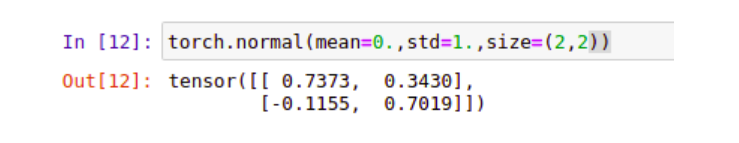
我们也可以让每一个值服从不同的正态分布,我们还是生成2x2的矩阵:
torch.normal(mean=torch.arange(4.),std=torch.arange(1.,0.6,-0.1)).reshape(2,2)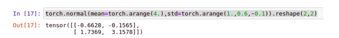
max
pred = torch.tensor([[0.7,0,0.2,0.1,0],[0,0.2,0.4,0.3,0.1]])
a = pred.max(1, keepdim=True)
print(a)
print(a[1])
'''
torch.return_types.max(
values=tensor([[0.7000],
        [0.4000]]),
indices=tensor([[0],
        [2]]))

tensor([[0],
        [2]])

'''
sum
pred = torch.tensor([[0.7,0,0.2,0.1,0],									 [0,0.2,0.4,0.3,0.1]])
a = pred.sum(axis=1)
print(a) # tensor([1., 1.]),自动降维
a = pred.sum(axis=1,keepdim=True)
print(a)
'''
tensor([[1.],
        [1.]])
'''
detach()
detach() & data()
detach()返回一个新的tensor,是从当前计算图中分离下来的,但是仍指向原变量的存放位置,其grad_fn=None且requires_grad=False,得到的这个tensor永远不需要计算其梯度,不具有梯度grad,即使之后重新将它的requires_grad置为true,它也不会具有梯度grad。
clamp()
torch.clamp(input, min, max, out=None) → Tensor将输入input张量每个元素的夹紧到区间 [min ,max],,并返回结果到一个新张量。
操作定义如下
      | min, if x_i < min
y_i = | x_i, if min <= x_i <= max
      | max, if x_i > max
如果输入是FloatTensor or DoubleTensor类型,则参数min max 必须为实数,否则须为整数。【译注:似乎并非如此,无关输入类型,min, max取整数、实数皆可。】
参数:
- input (Tensor) – 输入张量
- min (Number) – 限制范围下限
- max (Number) – 限制范围上限
- out (Tensor, optional) – 输出张量
代码示例如下:
a=torch.randint(low=0,high=10,size=(10,1))
print(a)
a=torch.clamp(a,3,9)
print(a)

'''

tensor([[9.],
        [3.],
        [0.],
        [4.],
        [4.],
        [2.],
        [4.],
        [1.],
        [2.],
        [9.]])
tensor([[9.],
        [3.],
        [3.],
        [4.],
        [4.],
        [3.],
        [4.],
        [3.],
        [3.],
        [9.]])
'''
torch.distributions.Categorical
torch.distributions.Categorical 是 PyTorch 中的一个分布类,它表示具有固定类别概率的离散分布。使用 Categorical 类,您可以创建一个离散分布对象,其中每个类别的概率由输入的概率张量确定。
以下是一个使用 Categorical 类的示例:
import torch
from torch.distributions import Categorical

# 定义一个概率张量,表示三个类别的概率分别为 0.3、0.5 和 0.2
probs = torch.tensor([0.3, 0.5, 0.2])

# 创建一个 Categorical 分布对象
dist = Categorical(probs)

# 从分布中抽样
sample = dist.sample()
print(sample)  # 输出抽样结果,可能为 0、1 或 2

# 计算 log 概率密度函数
log_prob = dist.log_prob(sample)
print(log_prob)  # 输出 log 概率密度函数的值
在这里,我们首先定义了一个概率张量,其中三个类别的概率分别为 0.3、0.5 和 0.2。然后,我们使用 Categorical 类创建了一个分布对象 dist,其中每个类别的概率由概率张量 probs 确定。接着,我们使用 sample() 方法从分布中抽样,返回一个表示抽样结果的张量。最后,我们使用 log_prob() 方法计算抽样结果的对数概率密度函数的值。
需要注意的是,Categorical 类的概率张量必须是非负的,并且总和必须为 1。如果概率张量不满足这些条件,Categorical 类将引发异常。如果您的概率张量不满足这些条件,您可以使用 torch.softmax() 函数将其转换为满足条件的概率张量。
torch.stack
在pytorch中,常见的拼接函数主要是两个,分别是:
stack()cat()
实际使用中,这两个函数互相辅助,使用场景不同:关于cat()参考torch.cat(),但是本文主要说stack()。
函数的意义:使用stack可以保留两个信息:[1. 序列] 和 [2. 张量矩阵] 信息,属于【扩张再拼接】的函数。
形象的理解:假如数据都是二维矩阵(平面),它可以把这些一个个平面按第三维(例如:时间序列)压成一个三维的立方体,而立方体的长度就是时间序列长度。
该函数常出现在自然语言处理(NLP)和图像卷积神经网络(CV)中。
stack()
官方解释:沿着一个新维度对输入张量序列进行连接。 序列中所有的张量都应该为相同形状。
浅显说法:把多个2维的张量凑成一个3维的张量;多个3维的凑成一个4维的张量…以此类推,也就是在增加新的维度进行堆叠。
outputs = torch.stack(inputs, dim=?) → Tensor
参数
- inputs : 待连接的张量序列。
注:python的序列数据只有list和tuple。 - dim : 新的维度, 必须在
0到len(outputs)之间。
注:len(outputs)是生成数据的维度大小,也就是outputs的维度值。
重点
函数中的输入
inputs只允许是序列;且序列内部的张量元素,必须shape相等
—-举例:[tensor_1, tensor_2,..]或者(tensor_1, tensor_2,..),且必须tensor_1.shape == tensor_2.shape
dim是选择生成的维度,必须满足0<=dim<len(outputs);len(outputs)是输出后的tensor的维度大小
不懂的看例子,再回过头看就懂了。
- 例子
1.准备2个tensor数据,每个的shape都是[3,3]
# 假设是时间步T1的输出
T1 = torch.tensor([[1, 2, 3],
        		[4, 5, 6],
        		[7, 8, 9]])
# 假设是时间步T2的输出
T2 = torch.tensor([[10, 20, 30],
        		[40, 50, 60],
        		[70, 80, 90]])
2.测试stack函数
print(torch.stack((T1,T2),dim=0).shape)
print(torch.stack((T1,T2),dim=1).shape)
print(torch.stack((T1,T2),dim=2).shape)
print(torch.stack((T1,T2),dim=3).shape)
# outputs:
torch.Size([2, 3, 3])
torch.Size([3, 2, 3])
torch.Size([3, 3, 2])
'选择的dim>len(outputs),所以报错'
IndexError: Dimension out of range (expected to be in range of [-3, 2], but got 3)可以复制代码运行试试:拼接后的tensor形状,会根据不同的dim发生变化。
| dim | shape |
|---|---|
| 0 | [2, 3, 3] |
| 1 | [3, 2, 3] |
| 2 | [3, 3, 2] |
| 3 | 溢出报错 |
总结
函数作用:
函数stack()对序列数据内部的张量进行扩维拼接,指定维度由程序员选择、大小是生成后数据的维度区间。存在意义:
在自然语言处理和卷及神经网络中, 通常为了保留–[序列(先后)信息] 和 [张量的矩阵信息] 才会使用stack。
函数存在意义?》》》
手写过RNN的同学,知道在循环神经网络中输出数据是:一个list,该列表插入了seq_len个形状是[batch_size, output_size]的tensor,不利于计算,需要使用stack进行拼接,保留–[1.seq_len这个时间步]和–[2.张量属性[batch_size, output_size]]。
PyTorch中惰性模块初始化
LazyLinear
LazyConv2d
torchvision models
torchvision is a package in the PyTorch ecosystem that provides various tools and utilities for working with computer vision tasks. One of the key features of torchvision is its pre-trained models, which are neural networks trained on large datasets such as ImageNet.
Here are some of the pre-trained models available in torchvision:
- AlexNet: a deep convolutional neural network (CNN) introduced in 2012, which was one of the first models to achieve high accuracy on the ImageNet dataset.
- VGG: a series of CNNs with varying depths, developed by the Visual Geometry Group at the University of Oxford.
- ResNet: a family of CNNs introduced in 2015 that includes skip connections, allowing the model to learn residual functions.
- Inception: a family of CNNs that use a combination of different convolutional filters at different scales.
- DenseNet: a CNN architecture that connects each layer to every other layer in a feed-forward fashion.
- MobileNet: a lightweight CNN designed for mobile and embedded applications.
- EfficientNet: a family of CNNs that use a compound scaling method to improve both accuracy and efficiency.
These models are often used as a starting point for transfer learning, where a pre-trained model is fine-tuned on a new dataset for a specific task. This can greatly reduce the amount of training data and time needed to achieve high performance on a new task.
torchvision models 中关于resnet34的具体使用方法
resnet34是torchvision中的一个预训练模型,是ResNet系列中的一个相对较小的模型。以下是使用resnet34进行预测的一个简单示例:
导入所需的库和模块。
import torch
import torchvision.transforms as transforms
import torchvision.models as models
from PIL import Image
初始化预训练模型。
model = models.resnet34(pretrained=True)加载并预处理要进行预测的图像。
img_path = 'path/to/image.jpg'

# 定义图像转换
transform = transforms.Compose([
    transforms.Resize(256),  # 调整图像大小为256x256
    transforms.CenterCrop(224),  # 中心裁剪为224x224
    transforms.ToTensor(),  # 将图像转换为张量
    transforms.Normalize(
        mean=[0.485, 0.456, 0.406],  # ImageNet数据集的均值
        std=[0.229, 0.224, 0.225]  # ImageNet数据集的标准差
    )
])

# 加载图像并进行转换
img = Image.open(img_path)
img_tensor = transform(img)
将输入数据传入模型进行推断。
# 将输入数据添加一个批次的维度
img_tensor = img_tensor.unsqueeze(0)

# 将模型设置为评估模式
model.eval()

# 通过模型进行推断
output = model(img_tensor)
在这个例子中,
img_path表示要进行预测的图像路径,transform表示对图像进行的预处理操作,例如调整大小、裁剪、归一化等。在传递给模型之前,需要将图像转换为张量并添加一个批次的维度。在推断之前,需要将模型设置为评估模式。推断之后,output表示模型的输出,是一个形状为[1, 1000]的张量,其中1000表示模型预测的类别数。可以使用torch.argmax(output)来获取预测结果的类别索引。
torchvision中的resnet34模型使用的默认输入通道为3(RGB彩色图像),输出通道为1000(对应ImageNet数据集中的1000个类别)。如果需要自己定义输入通道和输出通道,可以通过修改模型的构造函数实现。以下是一个简单的示例:
import torch.nn as nn
import torchvision.models as models

class ResNet34(nn.Module):
    def __init__(self, num_classes, input_channels=3):
        super(ResNet34, self).__init__()
        self.num_classes = num_classes
        self.input_channels = input_channels

        # 加载预训练模型
        self.model = models.resnet34(pretrained=True)

        # 替换第一层卷积层
        self.model.conv1 = nn.Conv2d(
            input_channels, 64, kernel_size=7, stride=2, padding=3, bias=False)

        # 替换最后一层全连接层
        self.model.fc = nn.Linear(512, num_classes)

    def forward(self, x):
        x = self.model(x)
        return x
在上面的示例中,我们首先定义了一个新的ResNet34类,它继承自nn.Module。在构造函数中,我们使用super()函数调用父类的构造函数,同时定义了num_classes和input_channels两个参数。在构造函数中,我们首先加载了resnet34预训练模型,然后替换了其第一层卷积层和最后一层全连接层,以适应自定义的输入通道和输出通道。
具体地,我们通过self.model.conv1来替换模型的第一层卷积层,这里我们使用了nn.Conv2d来定义新的卷积层,将其输入通道数设为input_channels,输出通道数设为64。类似地,我们通过self.model.fc来替换模型的最后一层全连接层,将其输入通道数设为512(resnet34模型的最后一层卷积层的输出通道数),输出通道数设为num_classes。
最后,我们在forward()函数中调用self.model()来实现前向传播。可以使用该自定义模型来训练自己的数据集,如:
model = ResNet34(num_classes=10, input_channels=1) # 假设输入通道为灰度图像

# 在训练之前对模型进行设备设置
device = torch.device("cuda:0" if torch.cuda.is_available() else "cpu")
model.to(device)

# 定义损失函数和优化器
criterion = nn.CrossEntropyLoss()
optimizer = torch.optim.Adam(model.parameters(), lr=0.001)

# 训练模型
for epoch in range(num_epochs):
    for i, (images, labels) in enumerate(train_loader):
        images = images.to(device)
        labels = labels.to(device)

        optimizer.zero_grad()
        outputs =
pandas
API
drop
功能:删除数据集中多余的数据
DataFrame.drop(labels=None, axis=0, index=None, columns=None, level=None, inplace=False, errors='raise')
常用参数详解:
labels:待删除的行名or列名;
axis:删除时所参考的轴,0为行,1为列;
index:待删除的行名
columns:待删除的列名
level:多级列表时使用,暂时不作说明
inplace:布尔值,默认为False,这是返回的是一个copy;若为True,返回的是删除相应数据后的版本
errors一般用不到,这里不作解释
#构件一个数据集
df1=pd.DataFrame(np.arange(36).reshape(6,6),columns=list('ABCDEF'))
'1.删除行数据'
#下面两种删除方式是等价的,传入labels和axis 与只传入一个index 作用相同
df2=df1.drop(labels=0,axis=0)
df22=df1.drop(index=0)
#删除多行数据
df3=df1.drop(labels=[0,1,2],axis=0)
df33=df1.drop(index=[0,1,2])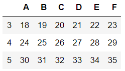
'2.删除列数据'
df4=df1.drop(labels=['A','B','C'],axis=1)
df44=df1.drop(columns=['A','B','C'])
'3.inplace参数的使用'
dfs=df1
#inplace=None时返回删除前的数据
dfs.drop(labels=['A','B','C'],axis=1)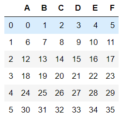
#inplace=True时返回删除后的数据
dfs.drop(labels=['A','B','C'],axis=1,inplace=True)
'4.drop函数在多级列表中的应用(实例copy自pandas官方帮助文档)‘
#构建多级索引
midx = pd.MultiIndex(levels=[['lama', 'cow', 'falcon'],
                             ['speed', 'weight', 'length']],
                     codes=[[0, 0, 0, 1, 1, 1, 2, 2, 2],
                            [0, 1, 2, 0, 1, 2, 0, 1, 2]])
#构造数据集
df = pd.DataFrame(index=midx, columns=['big', 'small'],
                  data=[[45, 30], [200, 100], [1.5, 1], [30, 20],
                        [250, 150], [1.5, 0.8], [320, 250],
                        [1, 0.8], [0.3, 0.2]])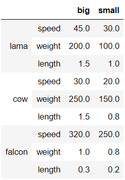
#同时删除行数据和列数据
df.drop(index='cow', columns='small')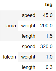
#删除某级index的对应行
df.drop(index='length',level=1)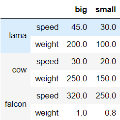
fillna
fillna(value=None, method=None, axis=None, inplace=False,limit=None, downcast=None, **kwargs)
value:用于填充的数值。method:表示填充方式,默认值为None。limit: 可以连续填充的最大数量,默认None。
method参数不能与value参数同时使用。
df = pd.DataFrame([[np.nan, 2, np.nan, 0],
                   [3, 4, np.nan, 1],
                   [np.nan, np.nan, np.nan, 5],
                   [np.nan, 3, np.nan, 4]],
                  columns=list("ABCD"))
df

'''
	A	B	C	D
0	NaN	2.0	NaN	0
1	3.0	4.0	NaN	1
2	NaN	NaN	NaN	5
3	NaN	3.0	NaN	4
'''
a_mean = df['A'].mean()
b_mean = df['B'].mean()
c_mean = df['C'].mean()
df.fillna({'A':a_mean,'B':b_mean,"C":c_mean},inplace=True)
df
'''
	A	B	C	D
0	3.0	2.0	NaN	0
1	3.0	4.0	NaN	1
2	3.0	3.0	NaN	5
3	3.0	3.0	NaN	4
'''
get_dummies
pd.get_dummies() 是 Pandas 的一个函数,它在一行代码中执行伪编码。数据科学家大多将其用于特征编码,但不建议将其用于生产或 Kaggle 竞赛。
==测试数据可能具有也可能不具有所有特征值,这可能会在建模时导致数据不匹配问题。==
pandas的get_dummies函数可以将分类数据转换为二进制哑变量(dummy variable)表示形式,方便机器学习和数据分析的处理。下面是get_dummies函数的用法:
pandas.get_dummies(data, prefix=None, prefix_sep='_', dummy_na=False, columns=None, sparse=False, drop_first=False, dtype=None)其中,参数说明如下:
data:要进行处理的DataFrame或Series对象。prefix:哑变量的列名前缀,用于与原始列进行区分。默认值为None,表示使用原始列名作为前缀。prefix_sep:前缀与列名的分隔符,默认值为下划线。dummy_na:是否为缺失值创建一列哑变量,如果为True,则将缺失值所在行的哑变量值设为1。默认值为False。columns:指定要进行哑变量转换的列,如果不指定,则默认对所有的分类数据进行处理。sparse:是否返回稀疏矩阵(SparseDataFrame),默认为False,表示返回密集矩阵(DataFrame)。drop_first:是否删除第一个哑变量列,默认为False,表示保留第一个哑变量列。dtype:指定输出矩阵的数据类型,默认为np.uint8。
下面是一个示例代码:
import pandas as pd

data = pd.DataFrame({'color': ['red', 'green', 'blue', 'red', 'blue']})
dummies = pd.get_dummies(data['color'], prefix='color')
data = pd.concat([data, dummies], axis=1)
print(data)
输出结果如下:
   color  color_blue  color_green  color_red
0    red           0            0          1
1  green           0            1          0
2   blue           1            0          0
3    red           0            0          1
4   blue           1            0          0
该示例代码将一列分类数据“color”转换为了三列哑变量数据,并将它们与原始数据进行合并。
import pandas as pd

data = pd.DataFrame({'color': ['red', 'green', 'blue', 'red', 'blue'],'age':[12,3,4,5,6]})
data = pd.get_dummies(data)
# data = pd.concat([data, dummies], axis=1)
print(data)
age color_blue color_green color_red
0 12 0 0 1
1 3 0 1 0
2 4 1 0 0
3 5 0 0 1
4 6 1 0 0to_numeric
pandas.to_numeric()是一个用于将Pandas对象(Series或DataFrame)中的数据转换为数值类型的函数。这个函数的语法如下:
pandas.to_numeric(arg, errors='raise', downcast=None)
其中,arg表示需要转换的Pandas对象,可以是一个Series或DataFrame,或是一个由Series或DataFrame构成的列表或字典;errors表示非数值数据的处理方式,它有以下几个选项:
'raise'(默认值):如果有非数值数据,就抛出异常;'coerce':如果有非数值数据,就将它们转换为NaN;'ignore':忽略非数值数据,不进行转换;
downcast表示转换后的数据类型,它可以是以下几个选项:
'integer':将数值类型转换为整型;'signed':将数值类型转换为带符号的整型;'unsigned':将数值类型转换为无符号的整型;'float':将数值类型转换为浮点型;
如果不指定downcast,则会根据转换后的数值类型自动选择合适的数据类型。
下面是一个示例代码,演示如何使用pandas.to_numeric()将Pandas对象中的数据转换为数值类型:
import pandas as pd

# 创建一个包含非数值数据的Series
s = pd.Series(['1', '2', '3a', '4b'])

# 将Series中的数据转换为数值类型
s = pd.to_numeric(s, errors='coerce')

# 输出结果
print(s)

'''
0    1.0
1    2.0
2    3.0
3    4.0
dtype: float64
'''
# 创建一个包含非数字元素的DataFrame
df = pd.DataFrame({'A': [1, 2, 3], 'B': [4, 5, 'fdfd']})

# 将列B中的非数字元素替换为NaN
df['B'] = pd.to_numeric(df['B'], errors='coerce')

# 输出结果
print(df)

'''
   A    B
0  1  4.0
1  2  5.0
2  3  NaN

'''
在上面的示例中,我们使用pd.to_numeric()方法将Series中的数据转换为数值类型。由于Series中包含非数值数据,我们将errors参数设置为'coerce',将非数值数据转换为NaN。最后,我们输出了处理后的Series。
需要注意的是,pandas.to_numeric()方法不能处理多个特征的情况,如果要处理多个特征,需要对每个特征进行单独的转换。另外,如果要将某一列中的非数字元素替换为指定的值,可以使用replace()方法。
select_dtypes
找到特定类型的列,返回一个索引
train_data.select_dtypes('object').columns数据预处理
创建一个人工数据集,并存储在CSV(逗号分隔值)文件
import os

os.makedirs(os.path.join('..', 'data'), exist_ok=True)
data_file = os.path.join('..', 'data', 'house_tiny.csv')
print(data_file)
with open(data_file, 'w') as f:
    f.write('NumRooms,Alley,Price\n')
    f.write('NA,Pave,127500\n')
    f.write('2,NA,106000\n')
    f.write('4,NA,178100\n')
f.write('NA,NA,140000\n')..\data\house_tiny.csv从创建的CSV文件中加载原始数据集
import pandas as pd

data = pd.read_csv(data_file)
data
NumRooms Alley Price
0 NaN Pave 127500
1 2.0 NaN 106000
2 4.0 NaN 178100
3 NaN NaN 140000为了处理缺失的数据,典型的方法包括插值法和删除法, 这里,我们将考虑插值法
inputs, outputs = data.iloc[:, 0:2], data.iloc[:, 2]# iloc:对数据进行位置索引,从而在数据表中提取出相应的数据。
inputs = inputs.fillna(inputs.mean())
print(inputs)
NumRooms Alley
0 3.0 Pave
1 2.0 NaN
2 4.0 NaN
3 3.0 NaN对于inputs中的类别值或离散值,我们将“NaN”视为一个类别
inputs = pd.get_dummies(inputs, dummy_na=True)
print(inputs)
NumRooms Alley_Pave Alley_nan
0 3.0 1 0
1 2.0 0 1
2 4.0 0 1
3 3.0 0 1现在inputs和outputs中的所有条目都是数值类型,它们可以转换为张量格式
import torch

X, y = torch.tensor(inputs.values), torch.tensor(outputs.values)
X, y
(tensor([[3., 1., 0.],
[2., 0., 1.],
[4., 0., 1.],
[3., 0., 1.]], dtype=torch.float64),
tensor([127500, 106000, 178100, 140000]))