写在之前
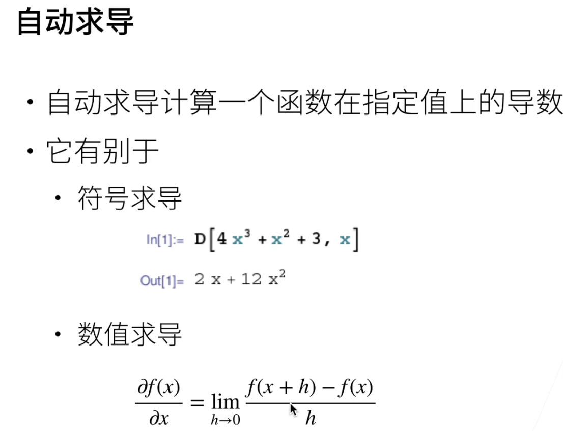
自动求导
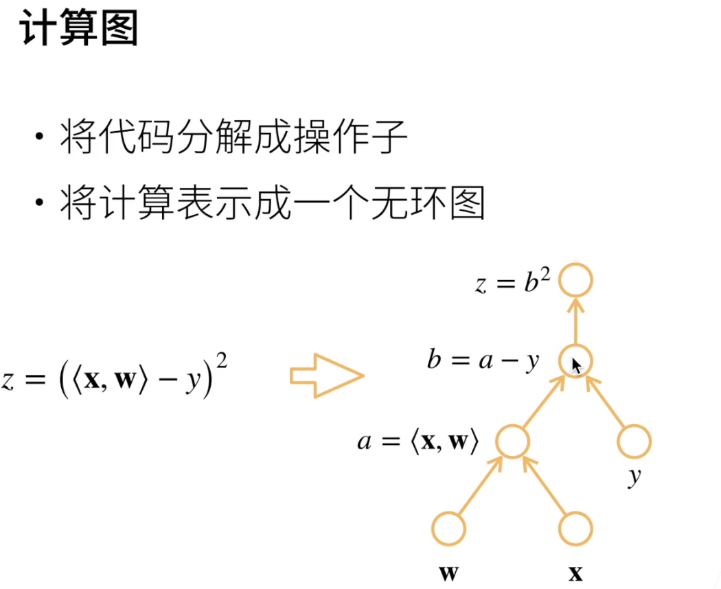
计算图可以显示的去构造
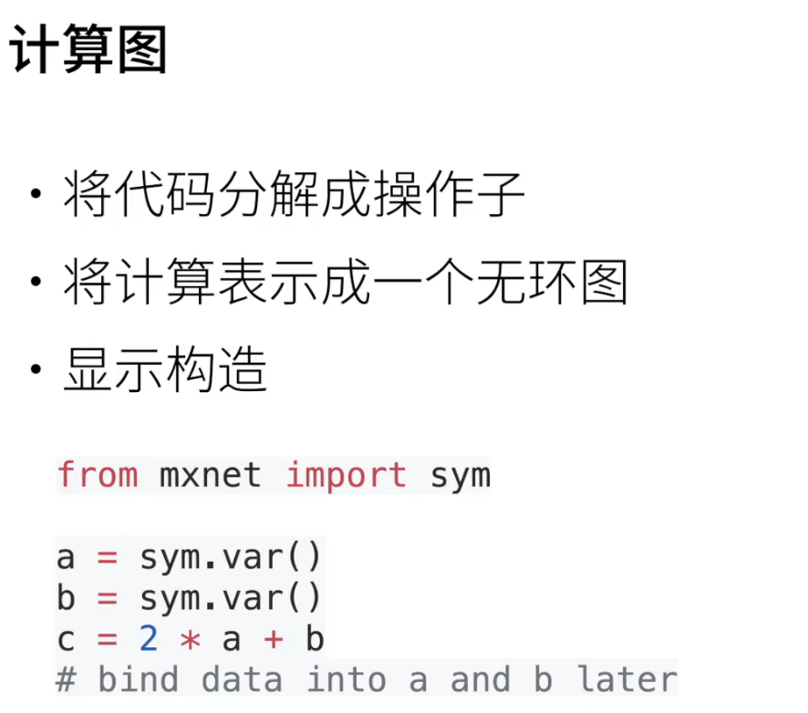
也可以隐式构造
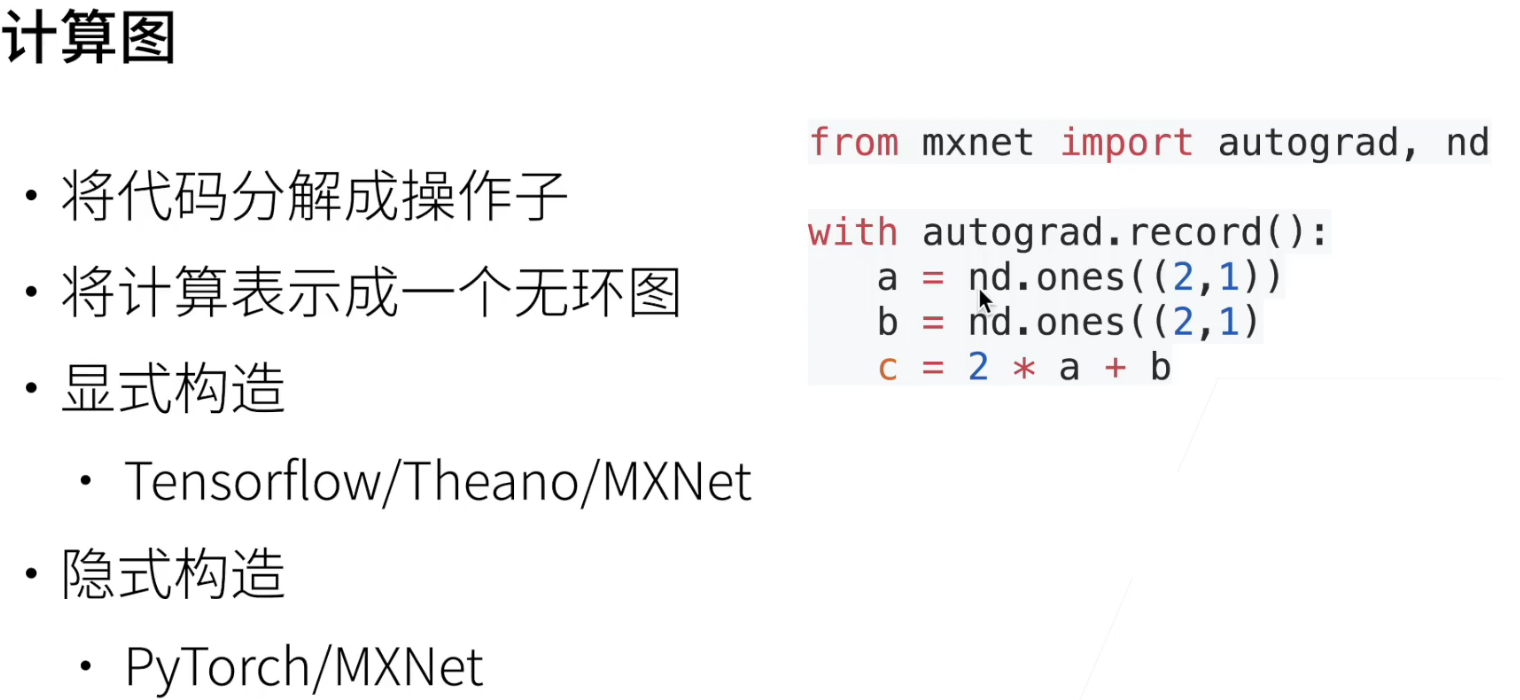
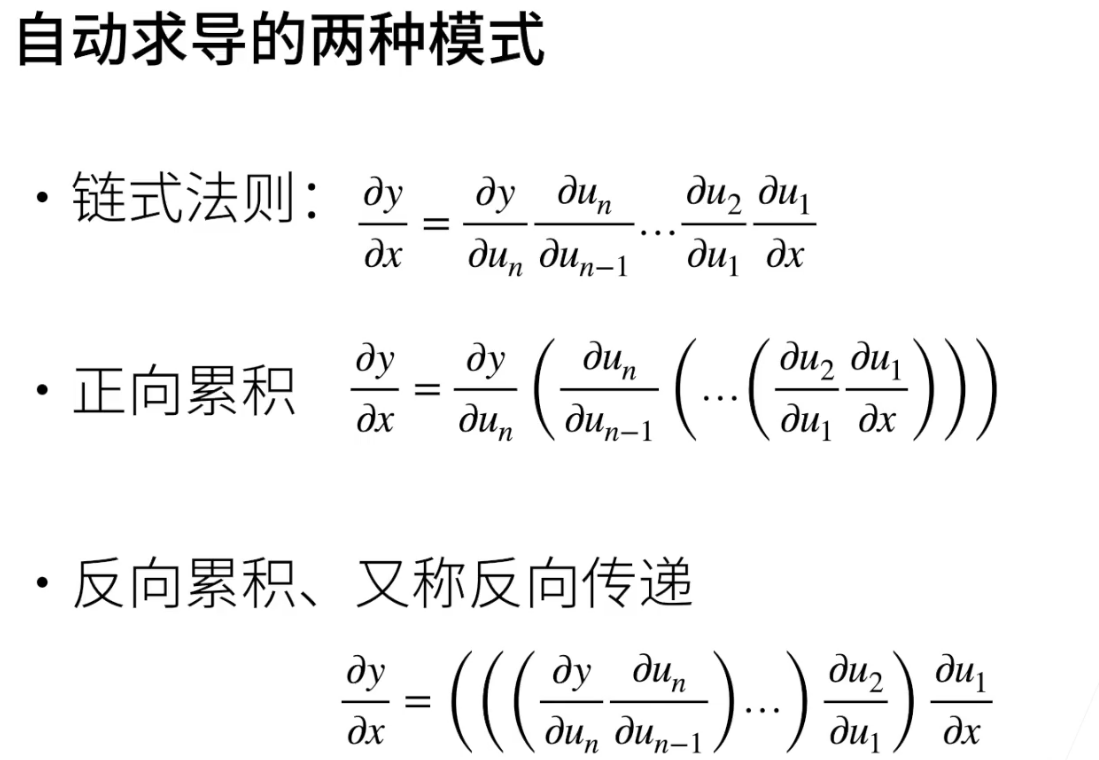
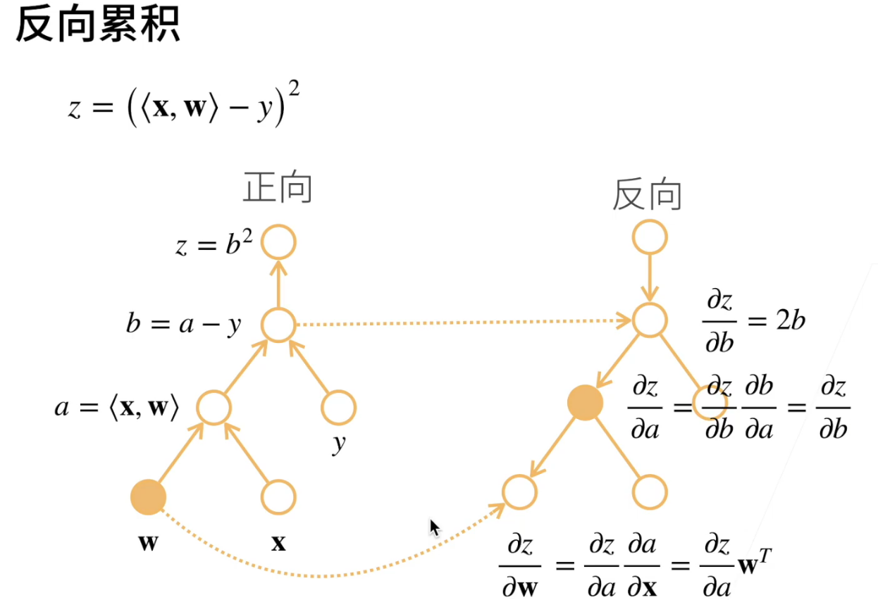
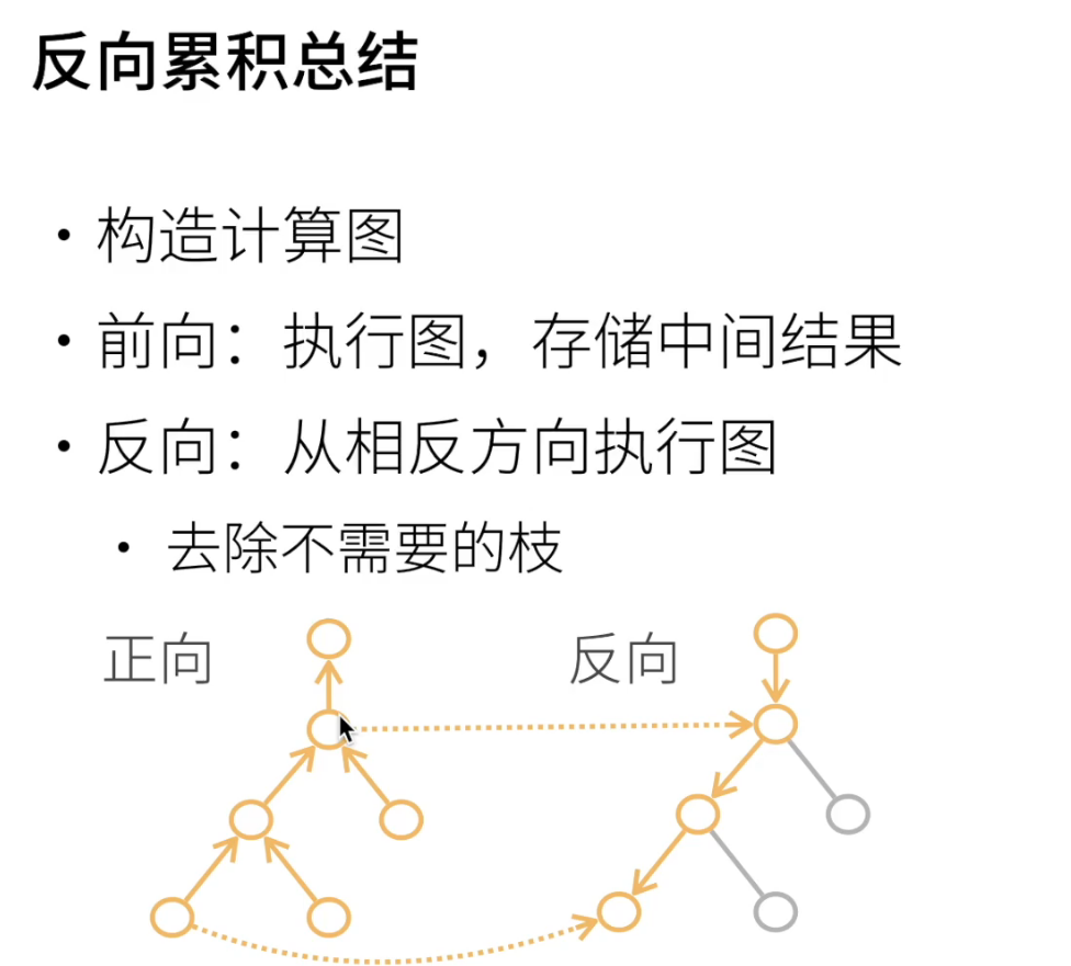
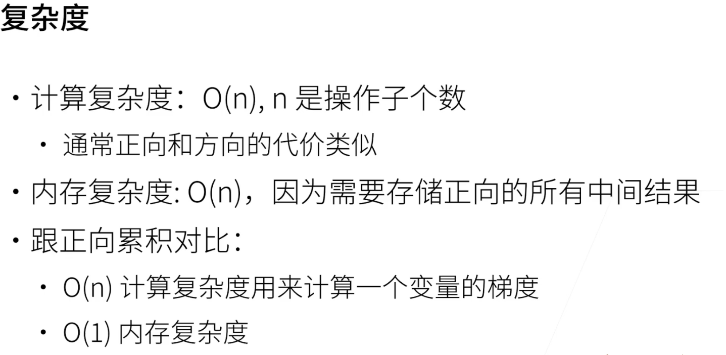
自动求导的两种方式:正向or反向
数据集
训练数据集
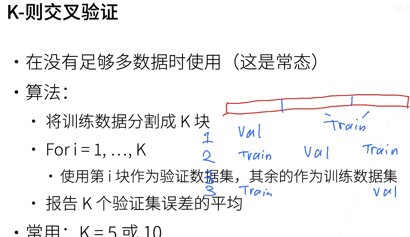
验证数据集
测试数据集
NOTE:
不要把验证数据集合测试数据集弄混
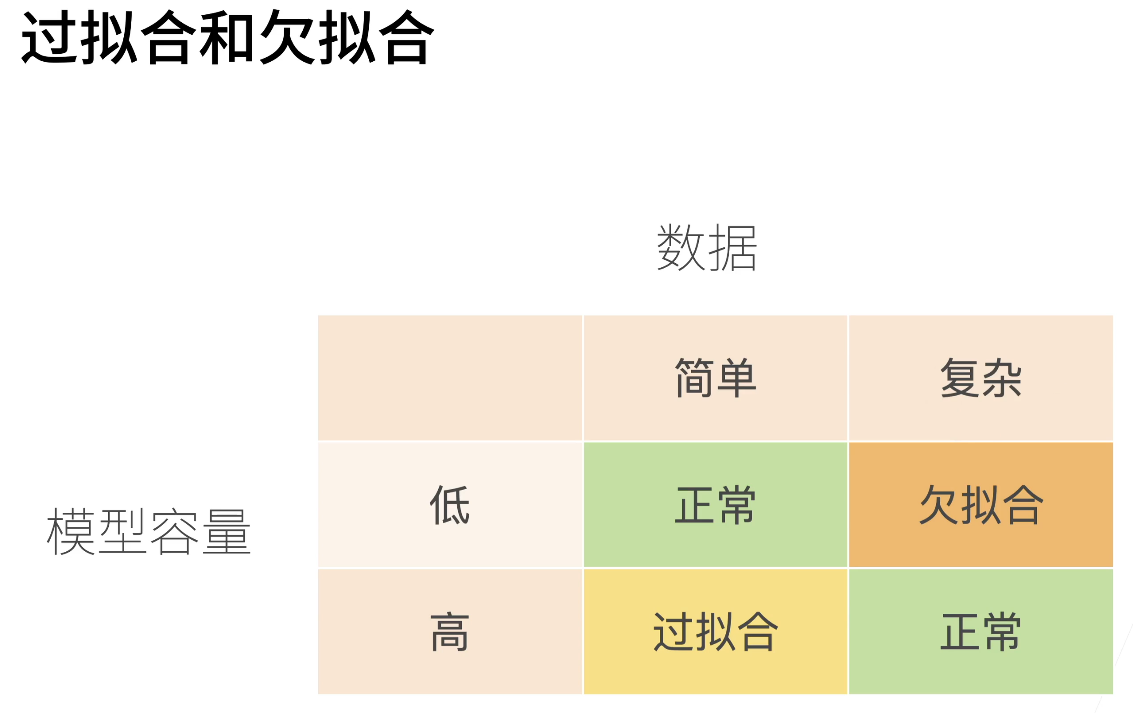
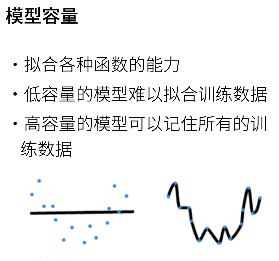
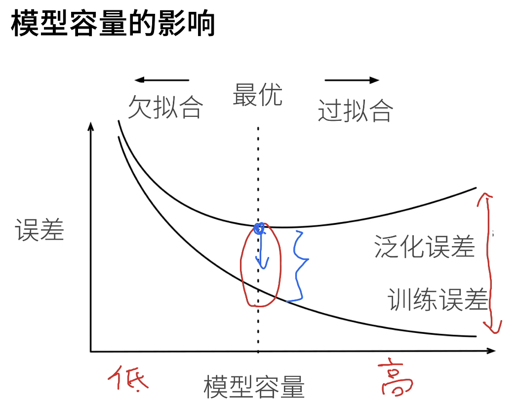
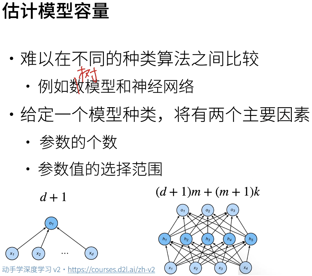
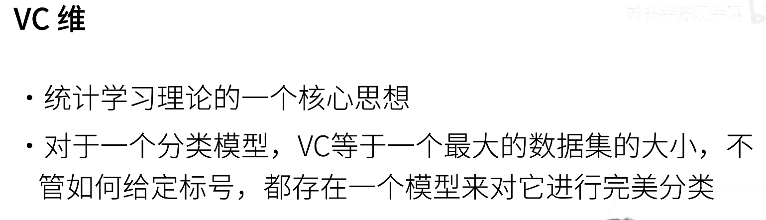
模型的选择以及过拟合和欠拟合
处理过拟合的方法
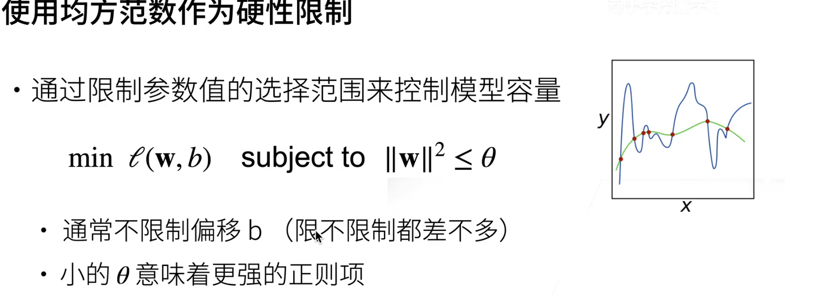
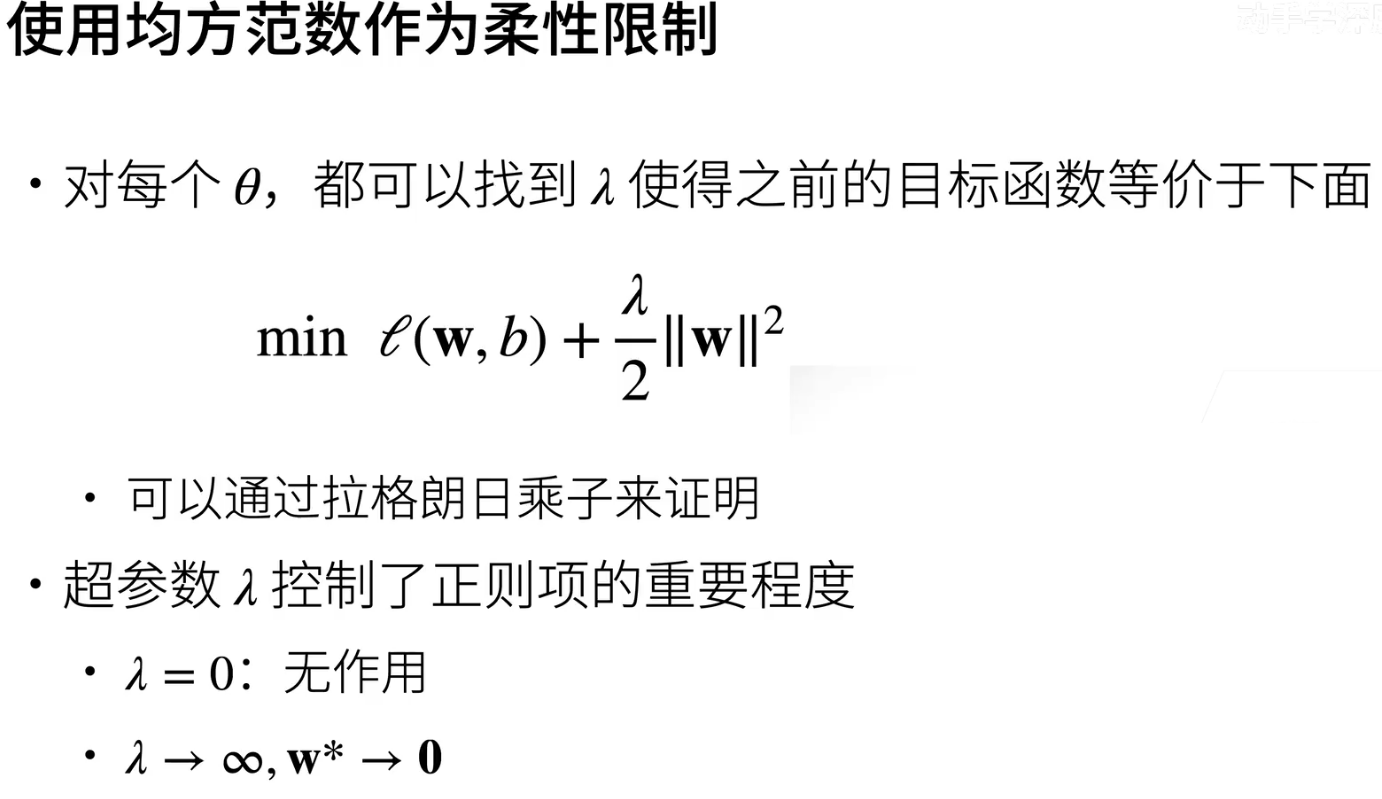
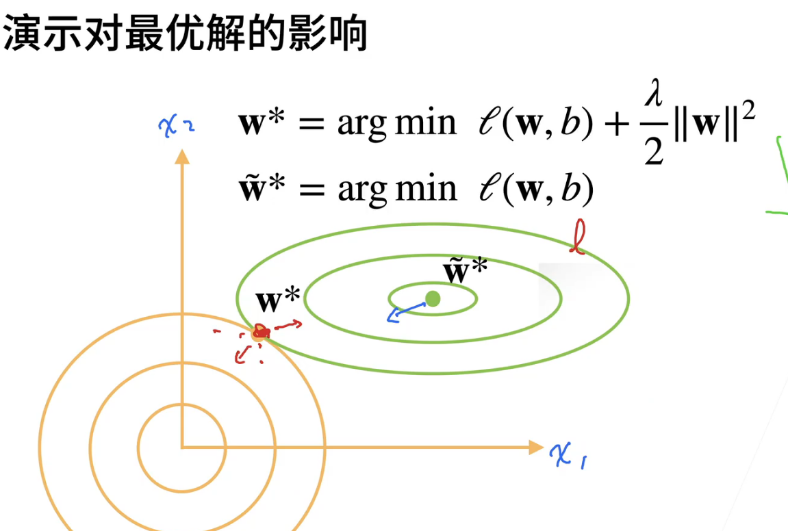
weight decay
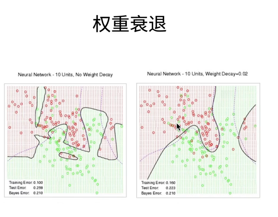
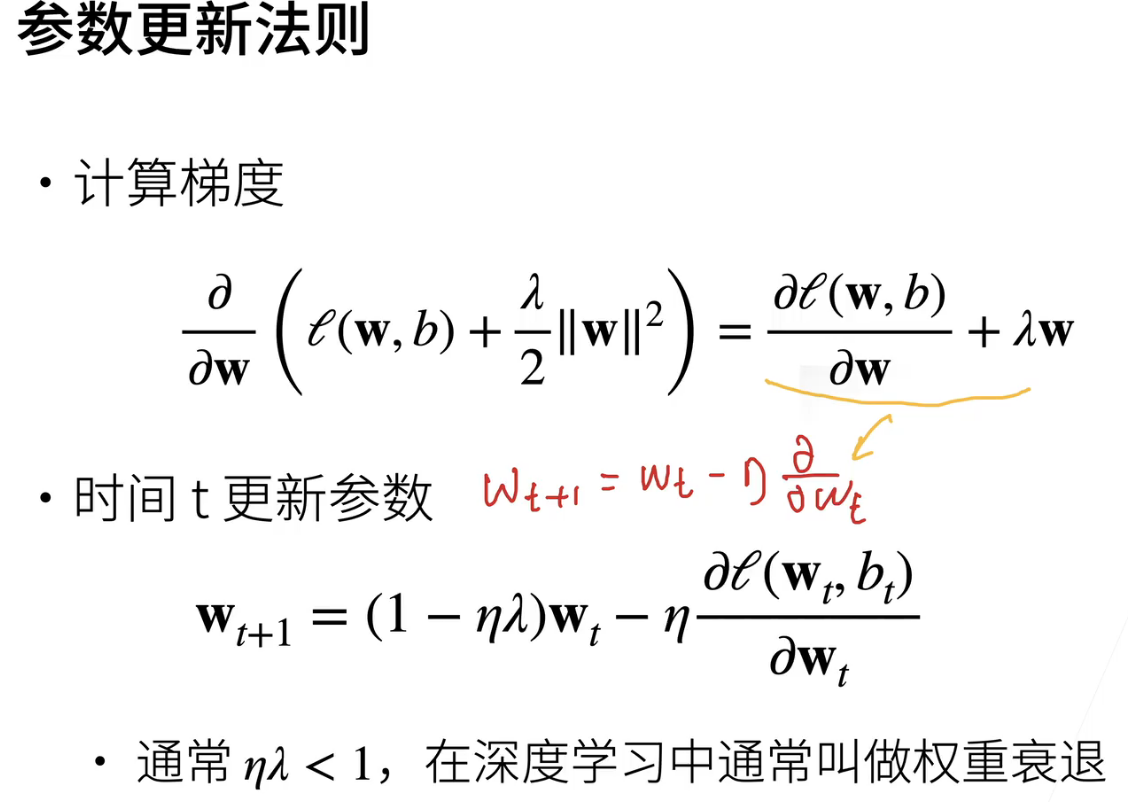
对$w_t$的权重衰减值往往设为1e-2/1e-3/1e-4(ps: 1-$\eta\lambda$)
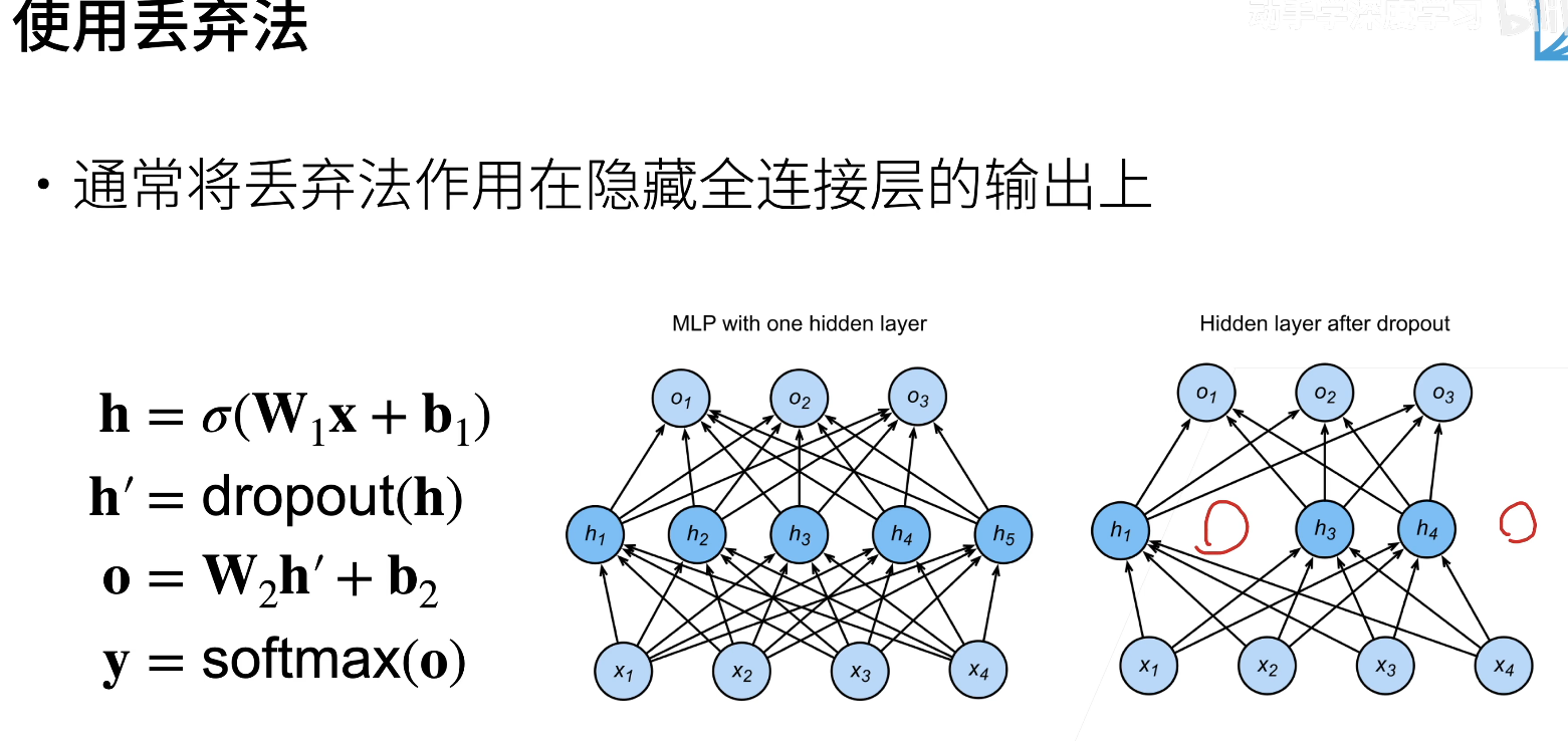
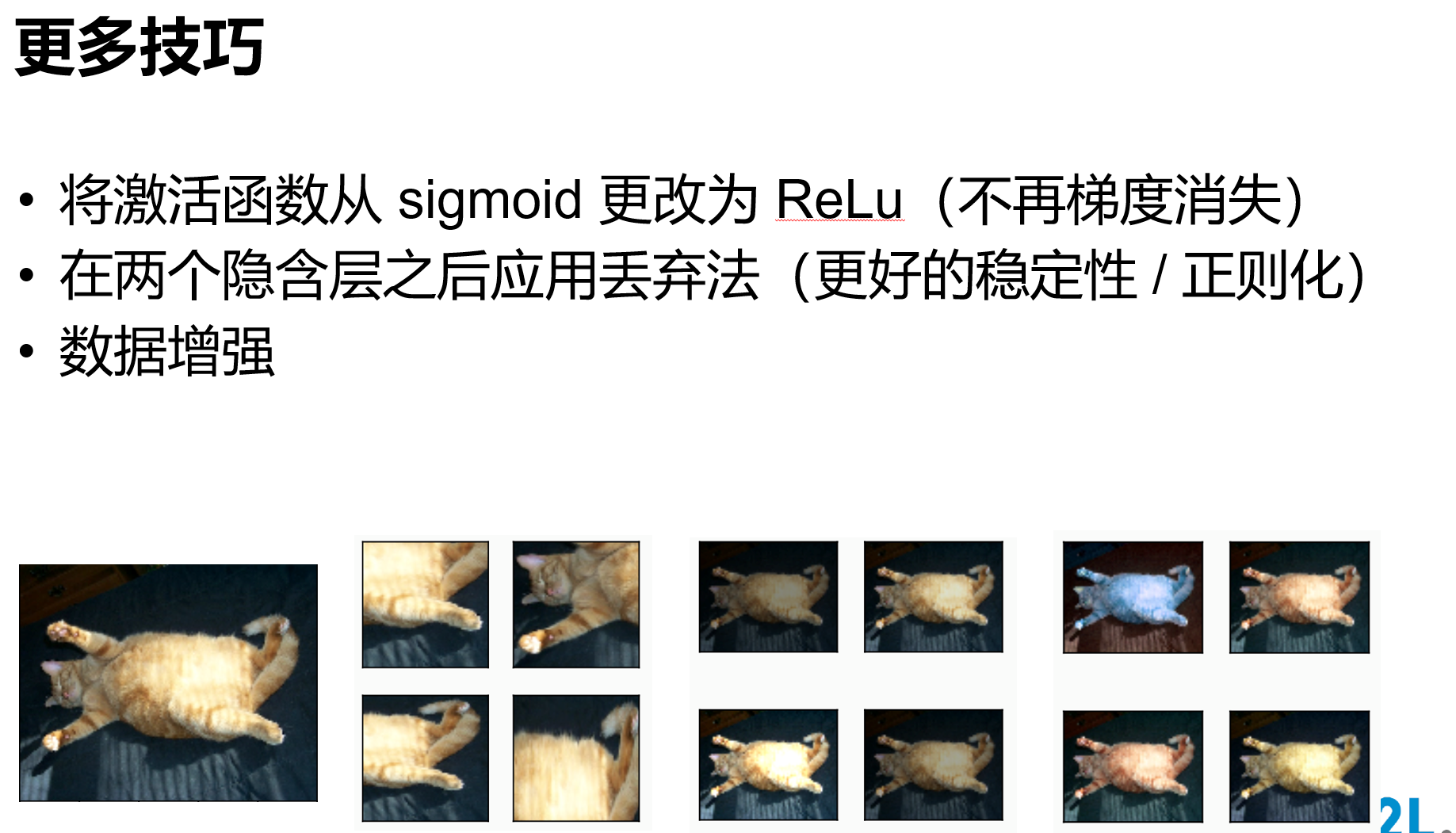
dropout(主流)
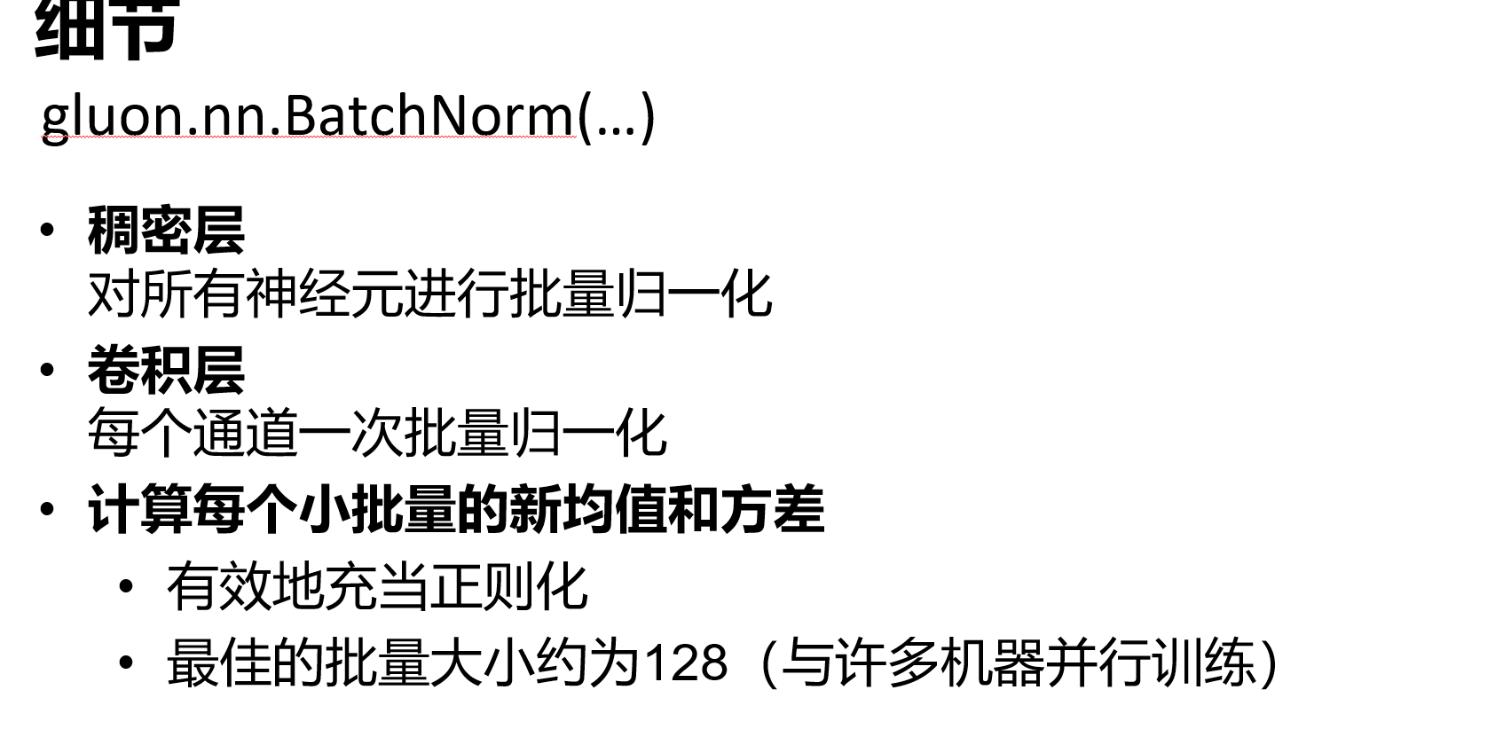
dropout用在全连接层,BN用在卷积层,两者不冲突
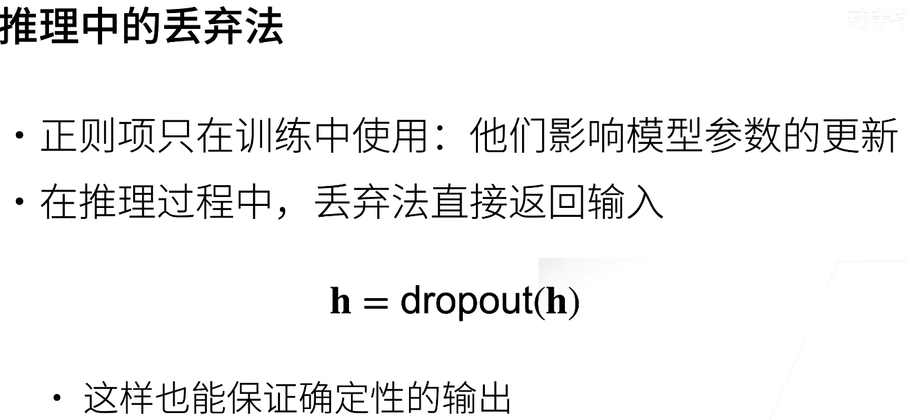
Dropout是一种常见的正则化方法,用来减少模型的复杂度

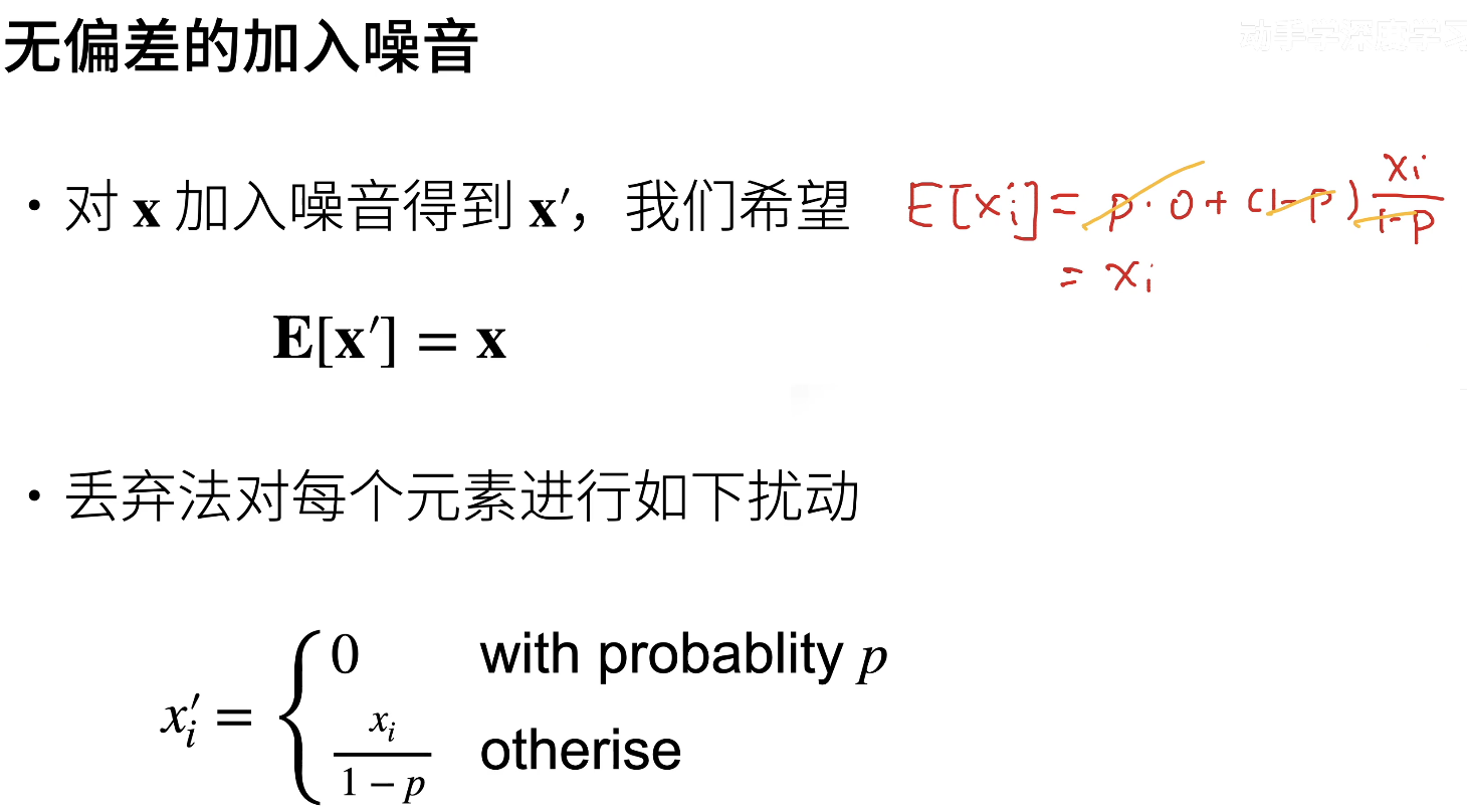
只在训练过程中使用正则方法,在测试过程(推理)中是不需要正则的
多用在多层感知机的隐藏层上,很少用在CNN之类的模型上
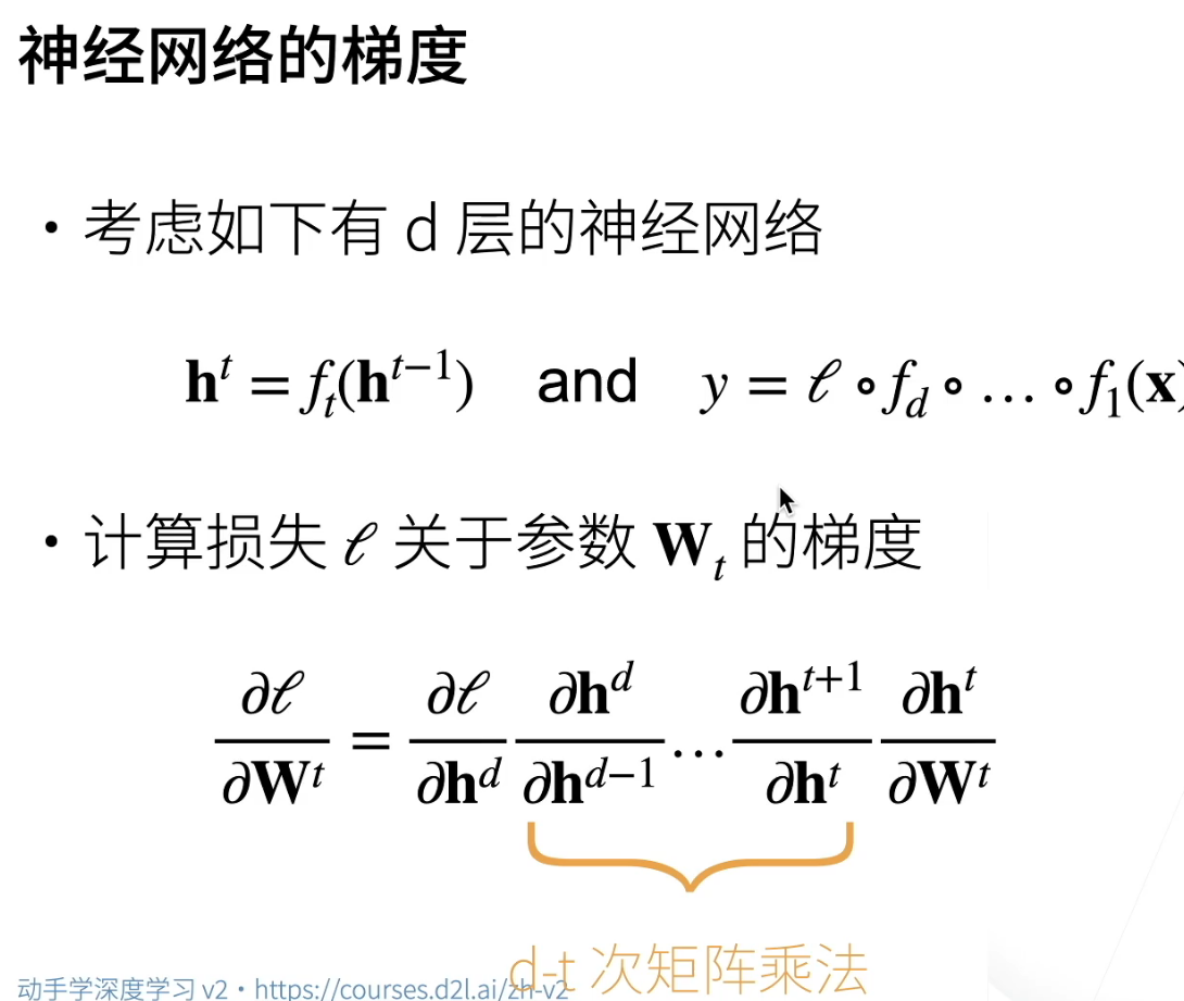
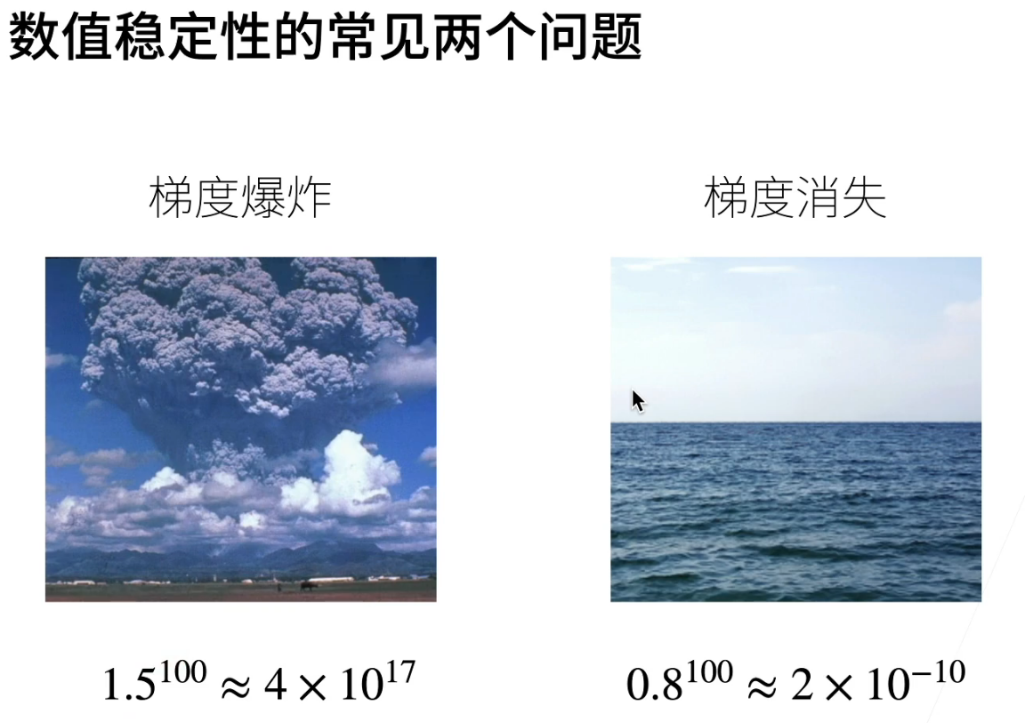
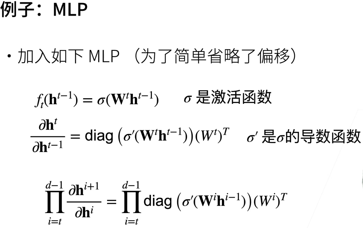
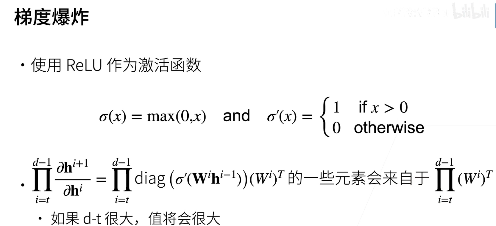
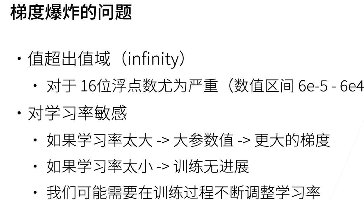
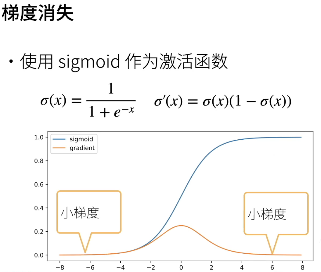
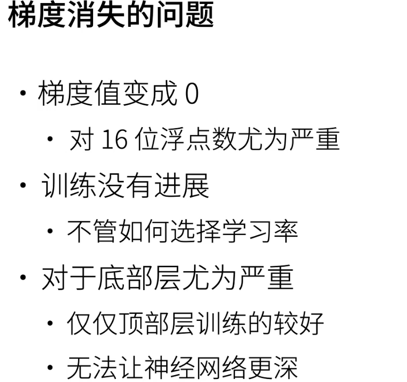
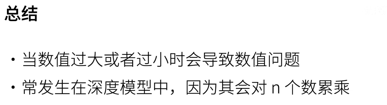
数值稳定性
梯度爆炸&梯度消失
用gpu训练时,我们往往会采用16位浮点数,因为训练速度上16位浮点数比32位浮点数快大约两倍
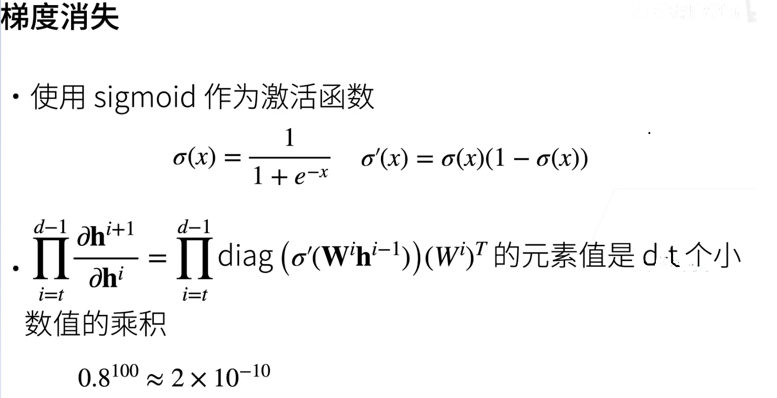
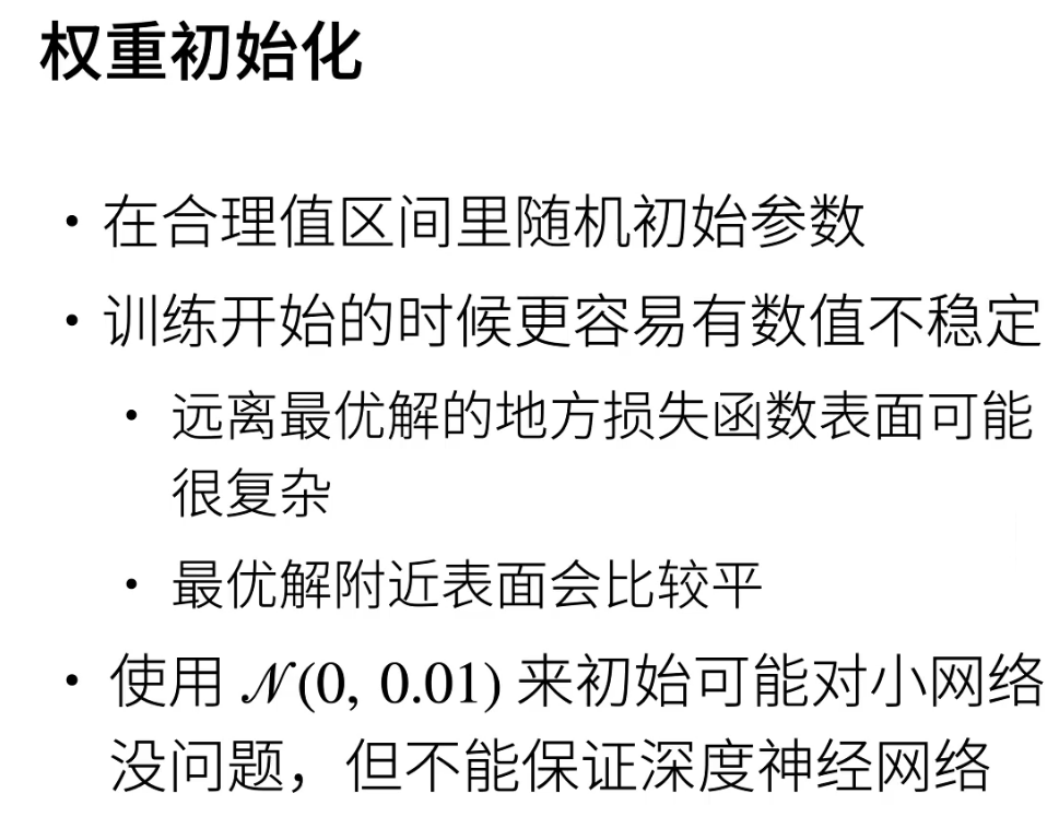
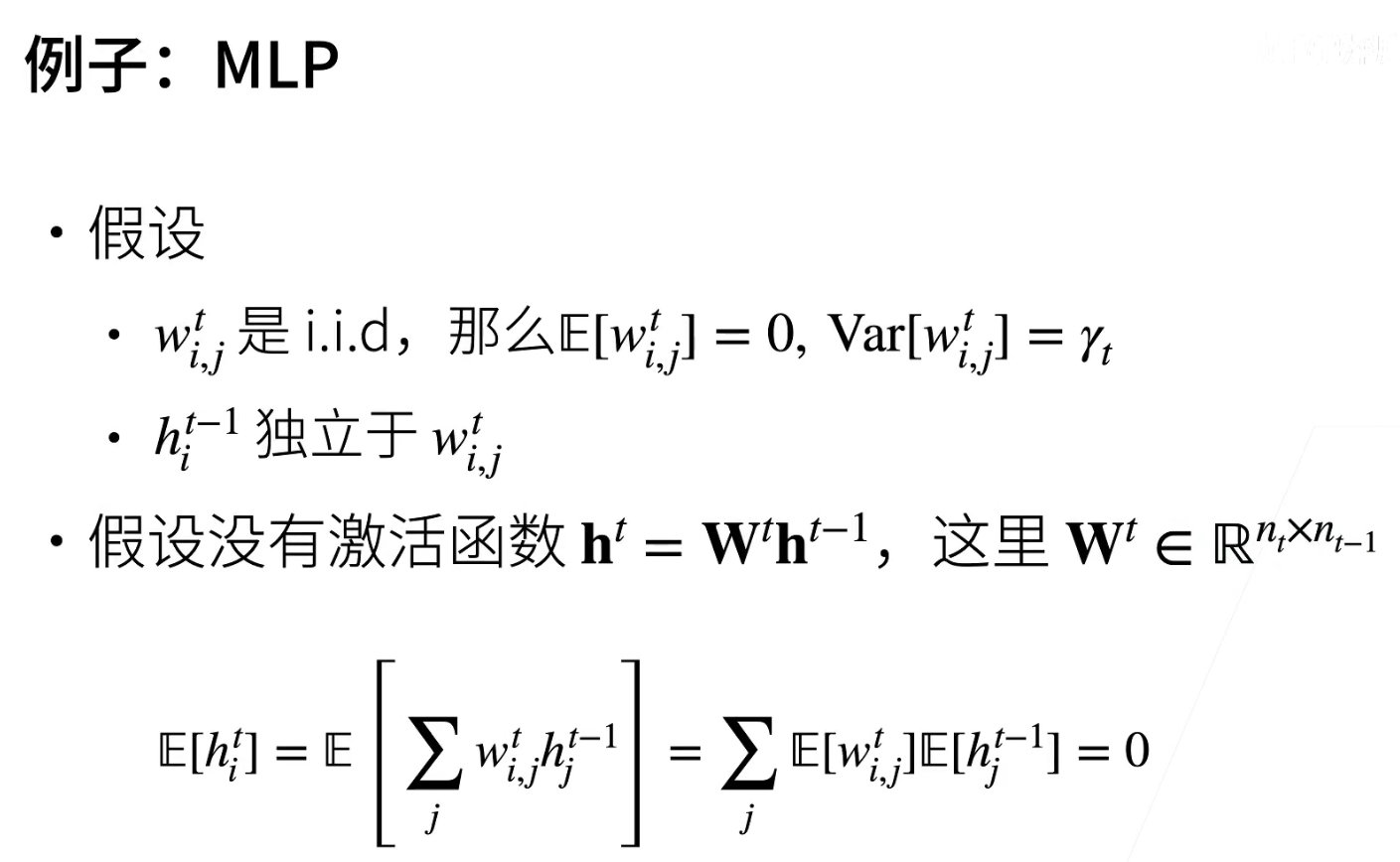
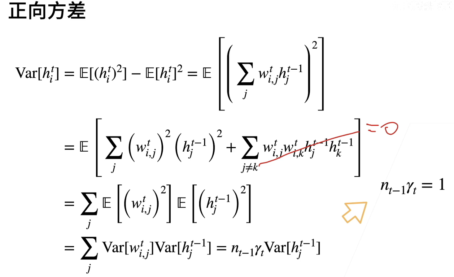
让训练更加稳定—模型初始化和激活函数
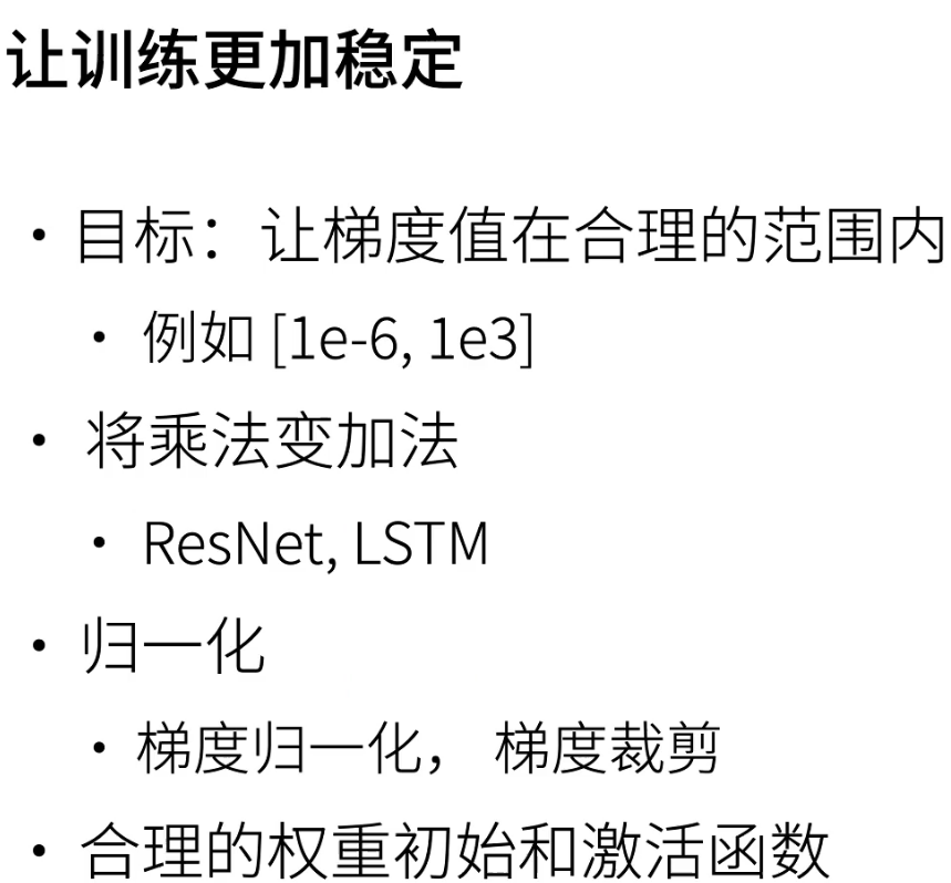
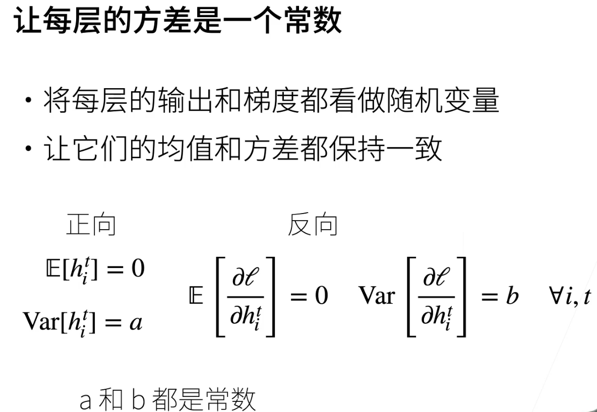
初始化是为了让训练不一开始就炸掉
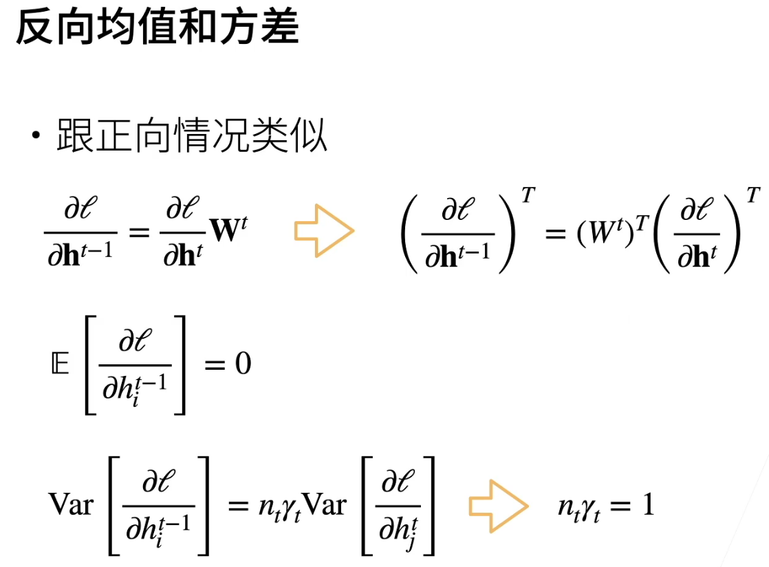
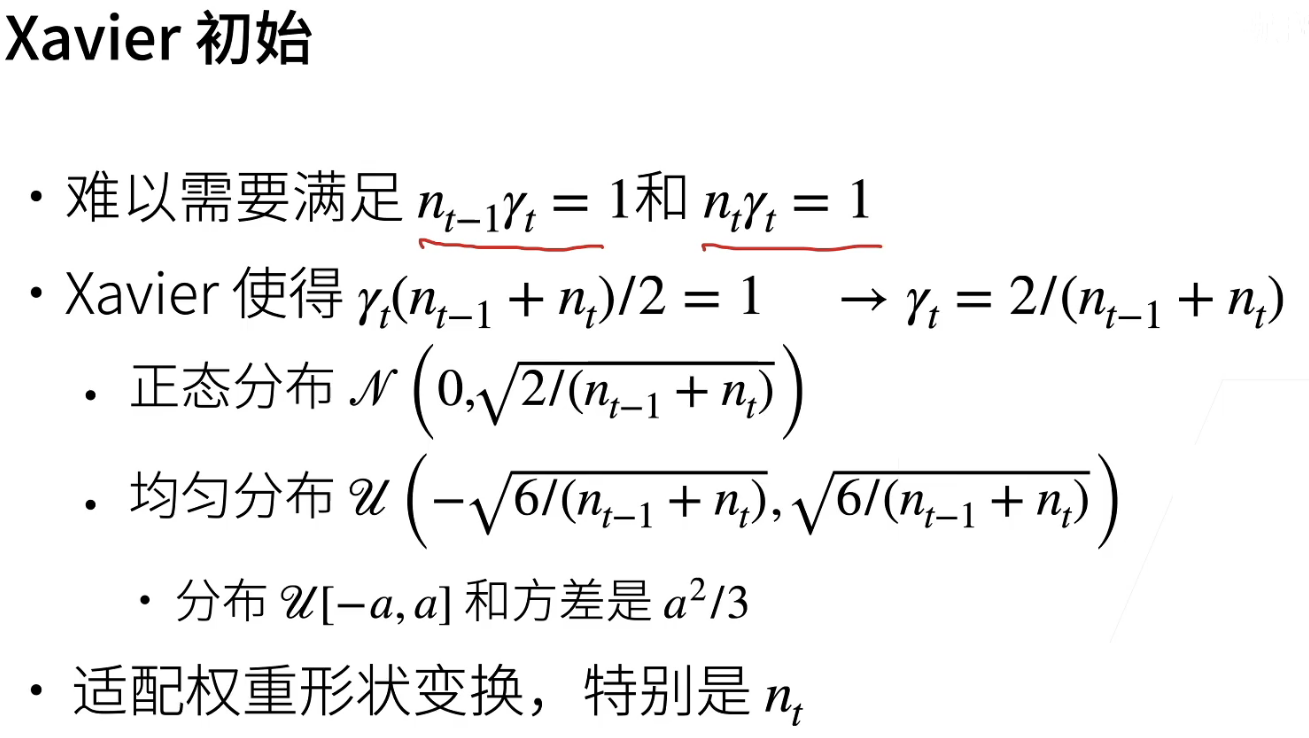
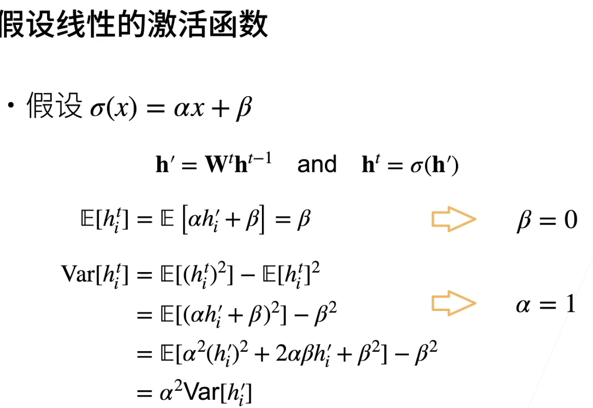
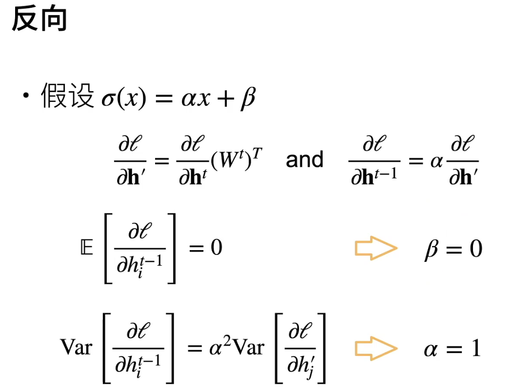
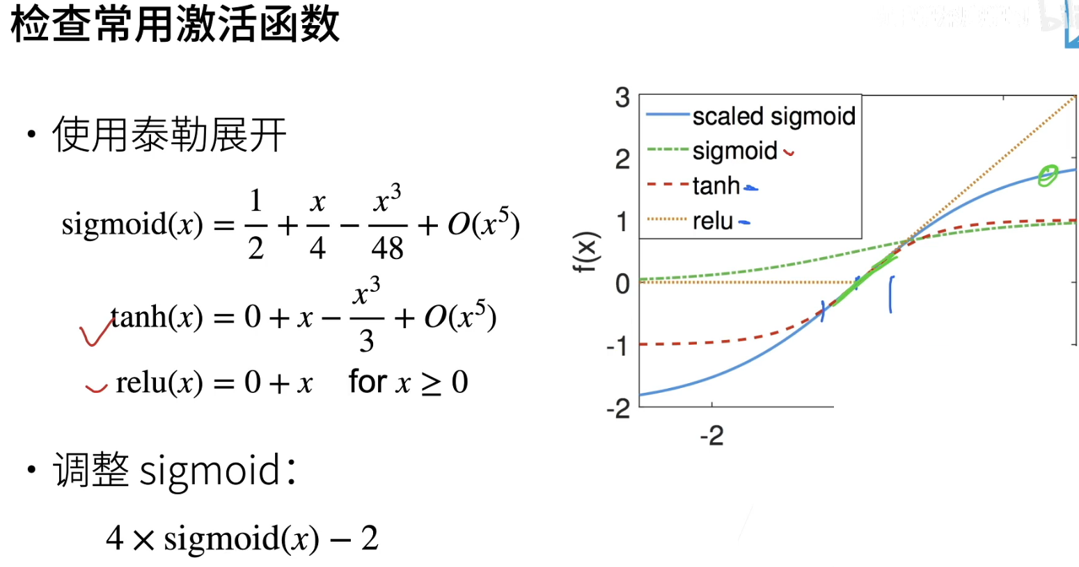
也就是说用xavier初始化权重,激活函数可以选择relu,tanh或者调整后的sigmoid
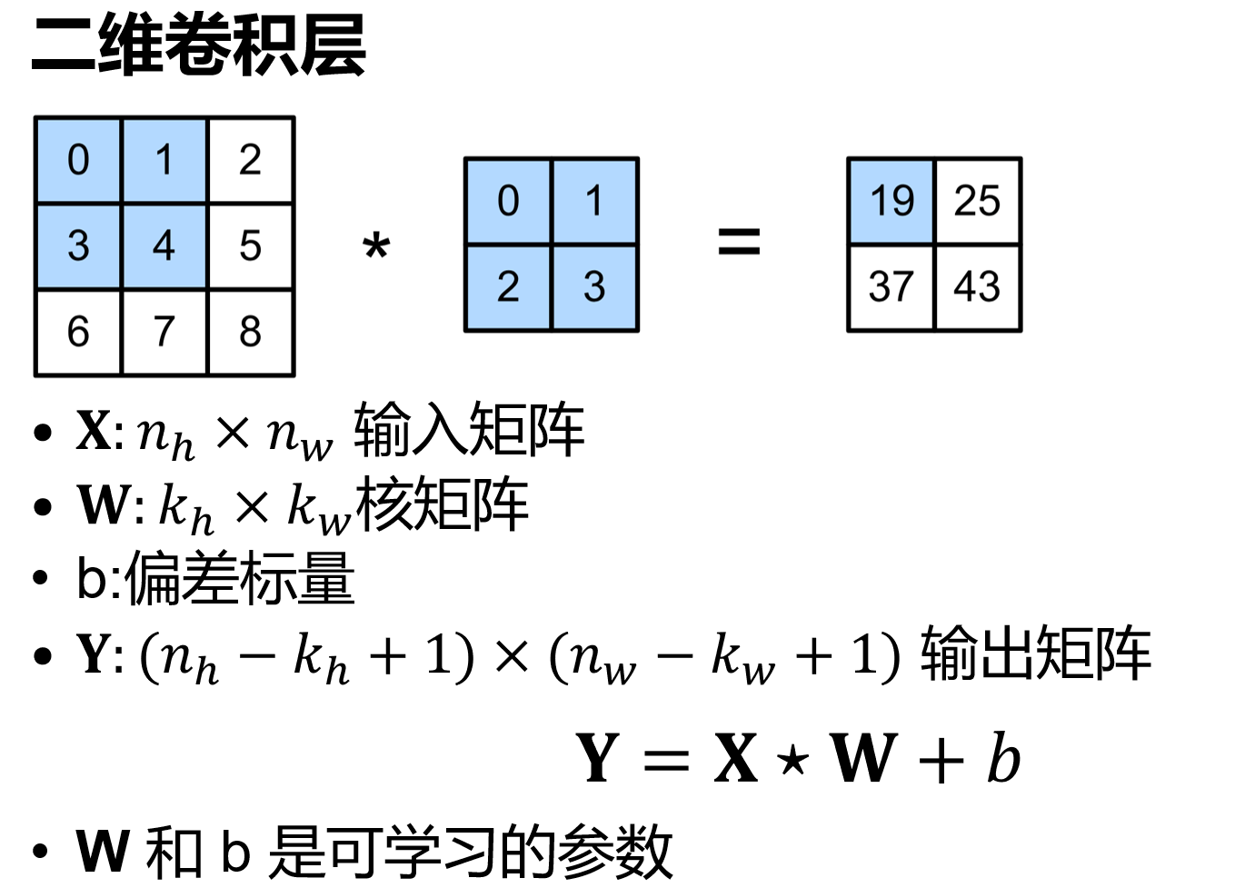
卷积层
卷积
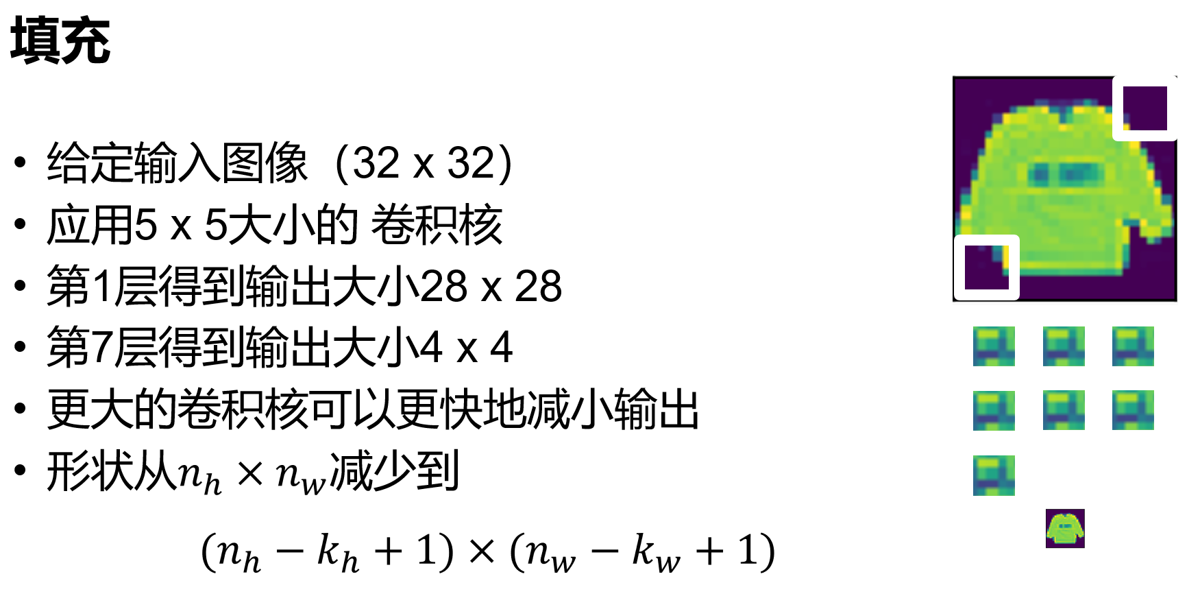
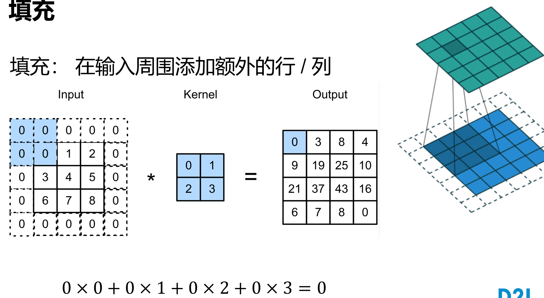
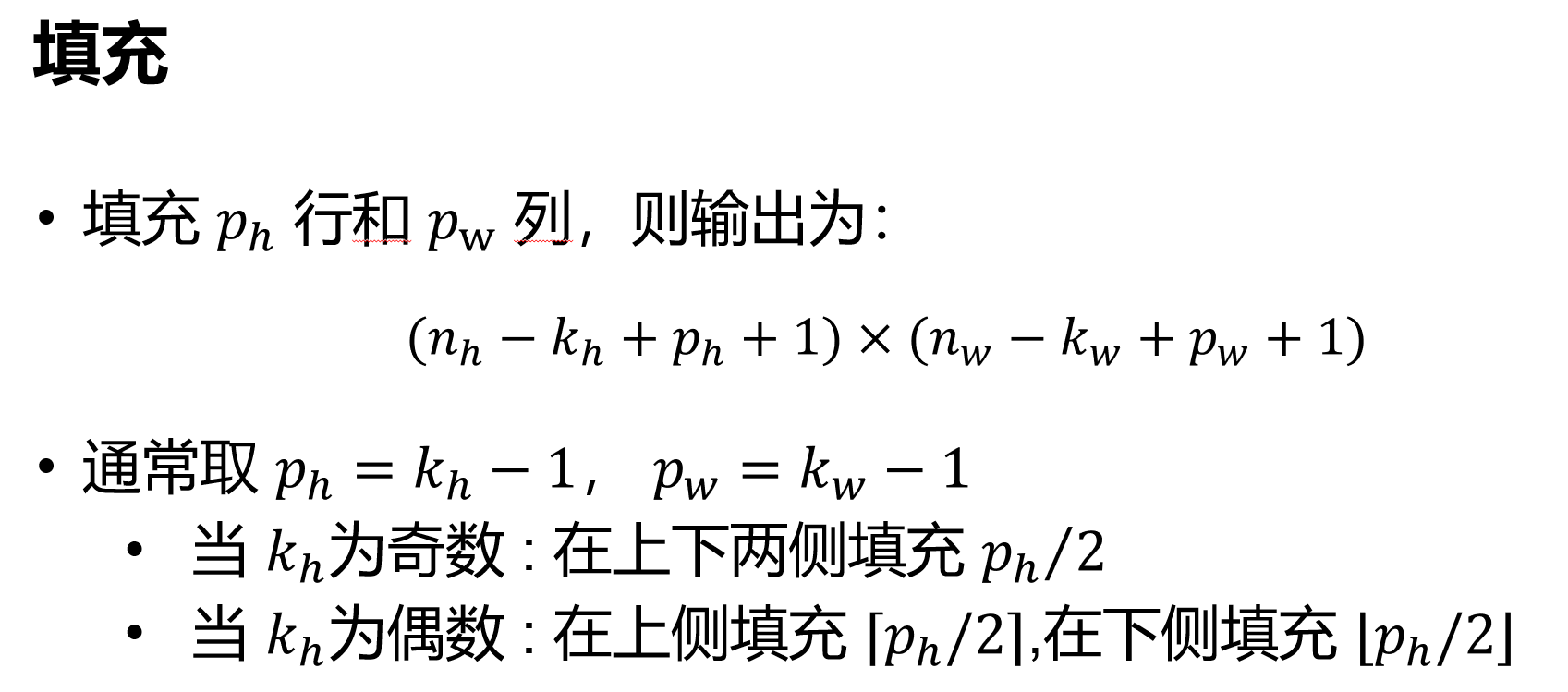
一般$p_h=k_h-1,p_w =k_w-1$
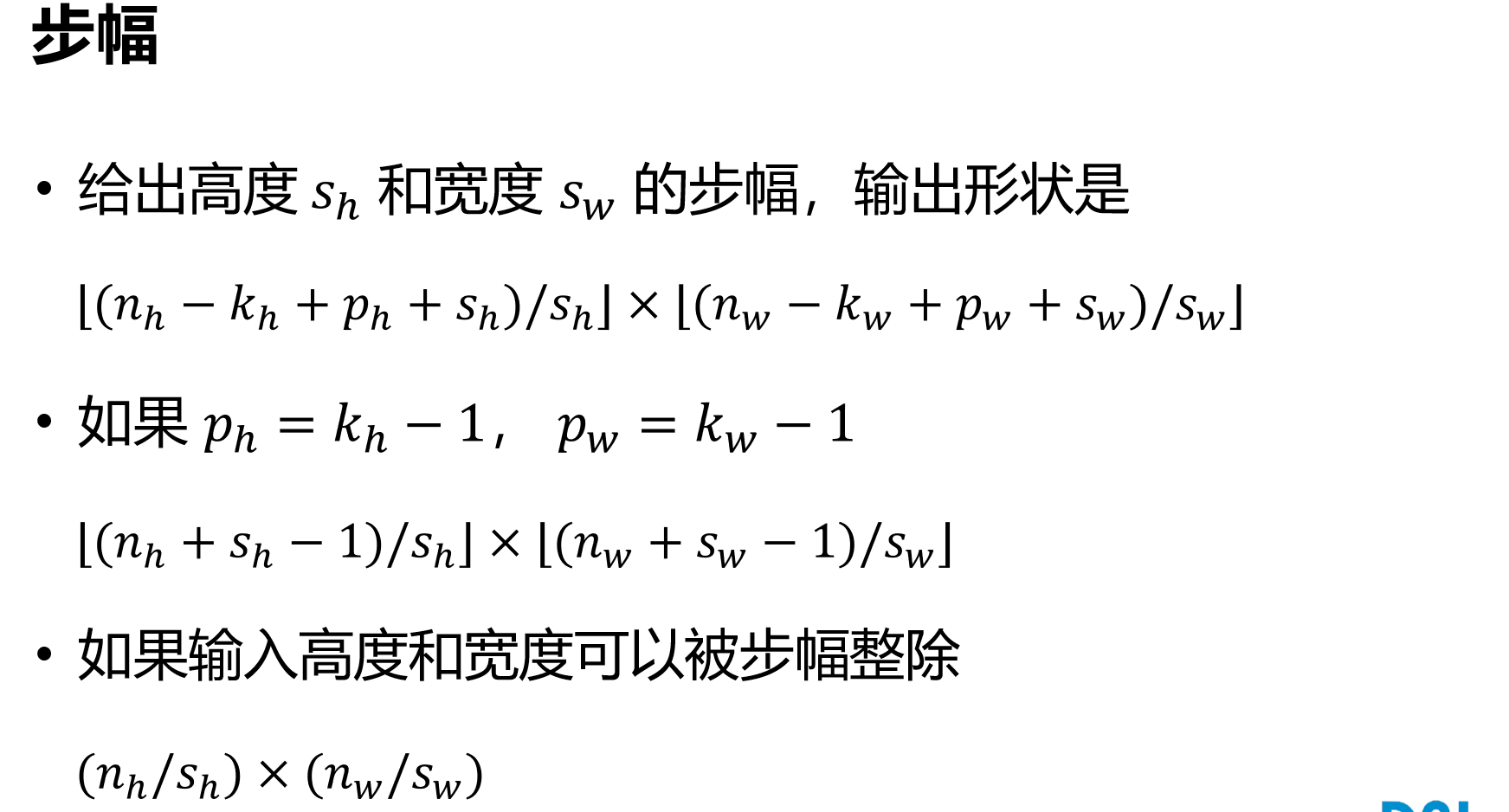
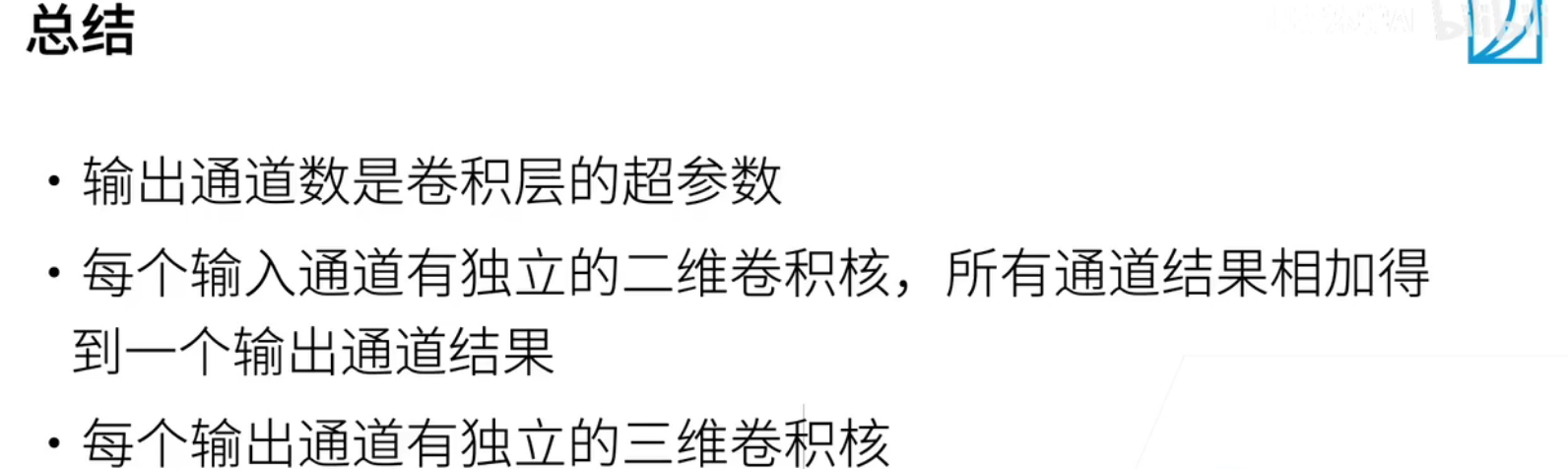
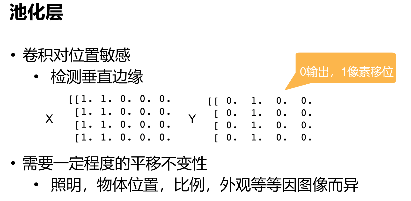
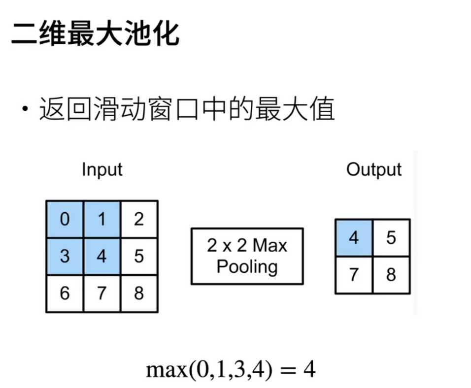
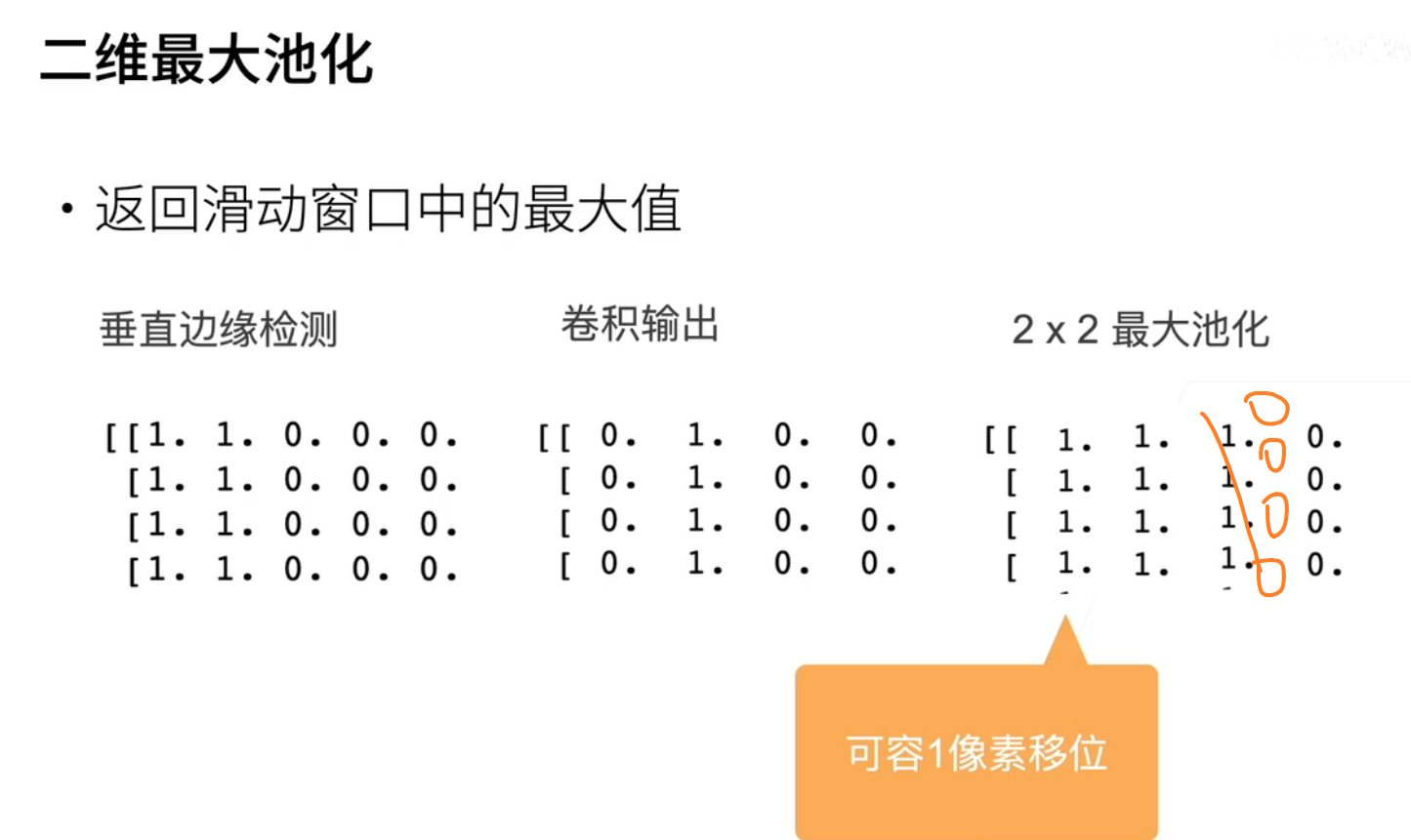
池化
池化输出的shape公式和卷积的类似
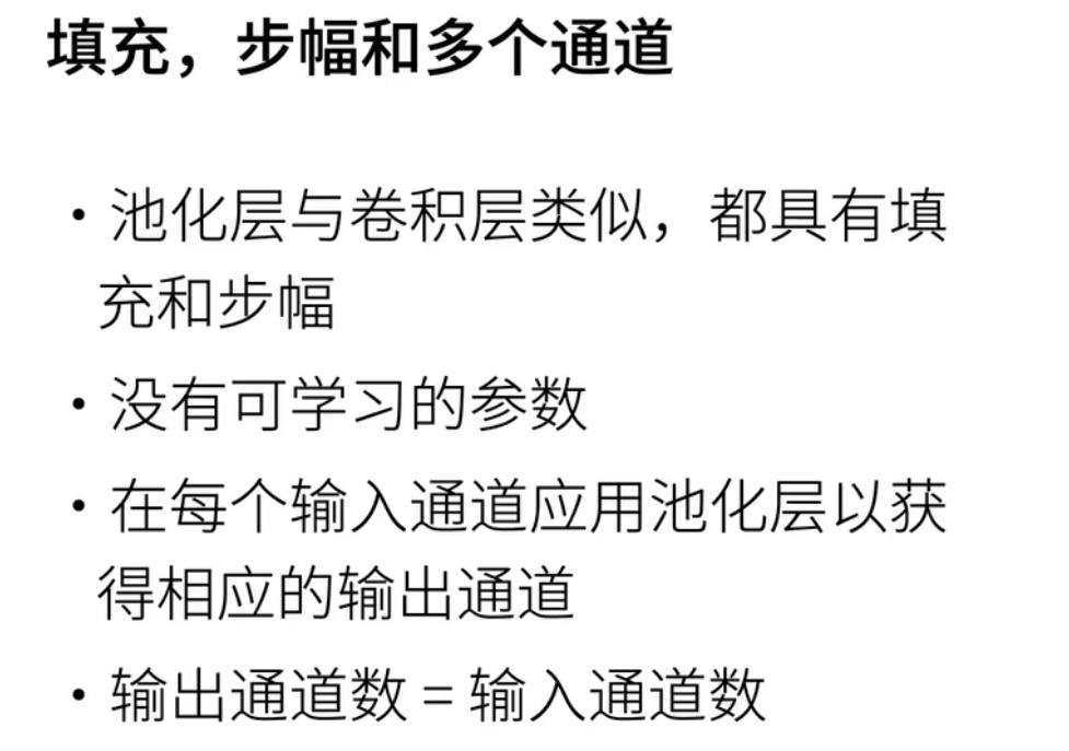

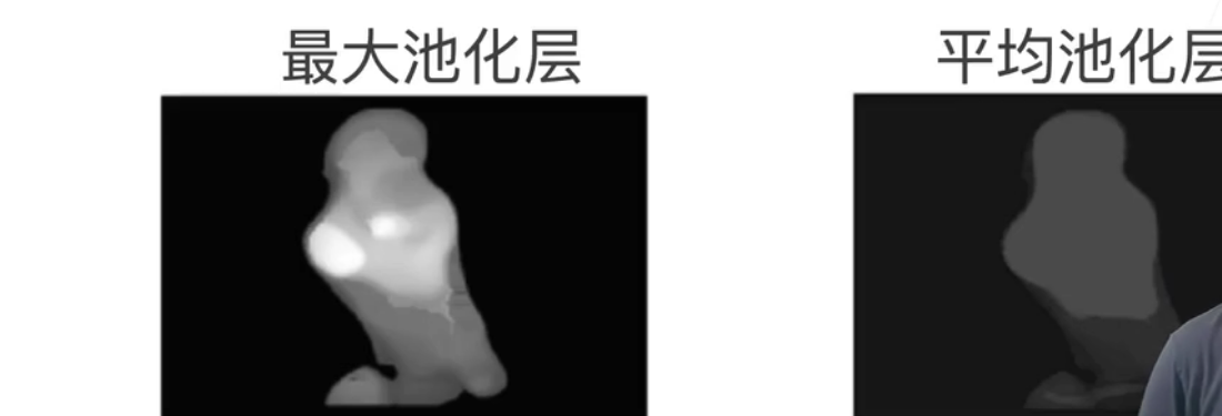
最大池化和平均 池化都是常用的操作
卷积神经网络模型
pytorch 中很多都已经集成了
torchvisionis a package in the PyTorch ecosystem that provides various tools and utilities for working with computer vision tasks. One of the key features oftorchvisionis its pre-trained models, which are neural networks trained on large datasets such as ImageNet.Here are some of the pre-trained models available in
torchvision:
- AlexNet: a deep convolutional neural network (CNN) introduced in 2012, which was one of the first models to achieve high accuracy on the ImageNet dataset.
- VGG: a series of CNNs with varying depths, developed by the Visual Geometry Group at the University of Oxford.
- ResNet: a family of CNNs introduced in 2015 that includes skip connections, allowing the model to learn residual functions.
- Inception: a family of CNNs that use a combination of different convolutional filters at different scales.
- DenseNet: a CNN architecture that connects each layer to every other layer in a feed-forward fashion.
- MobileNet: a lightweight CNN designed for mobile and embedded applications.
- EfficientNet: a family of CNNs that use a compound scaling method to improve both accuracy and efficiency.
These models are often used as a starting point for transfer learning, where a pre-trained model is fine-tuned on a new dataset for a specific task. This can greatly reduce the amount of training data and time needed to achieve high performance on a new task.
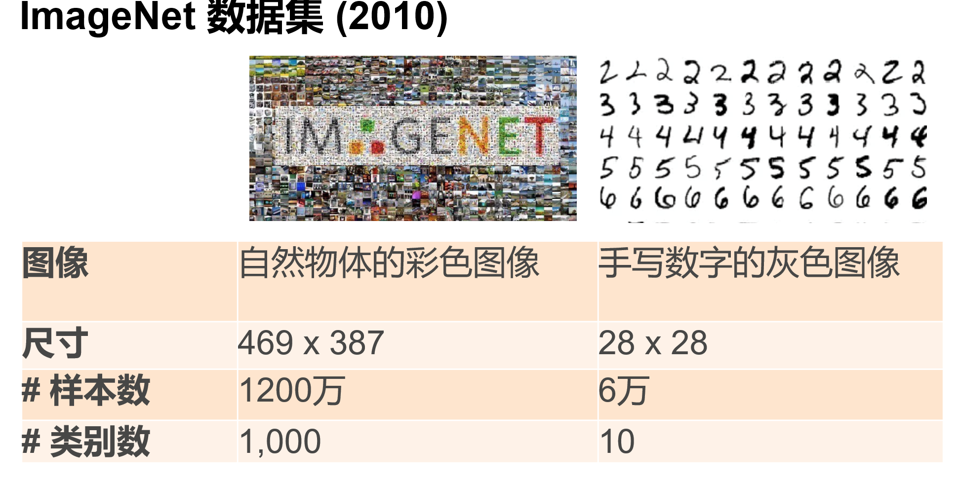
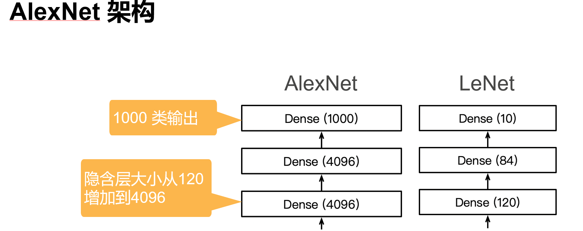
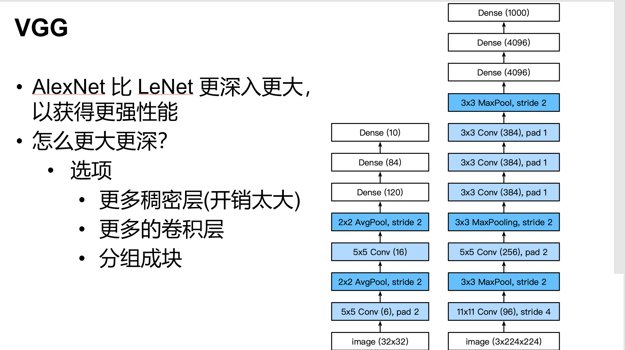
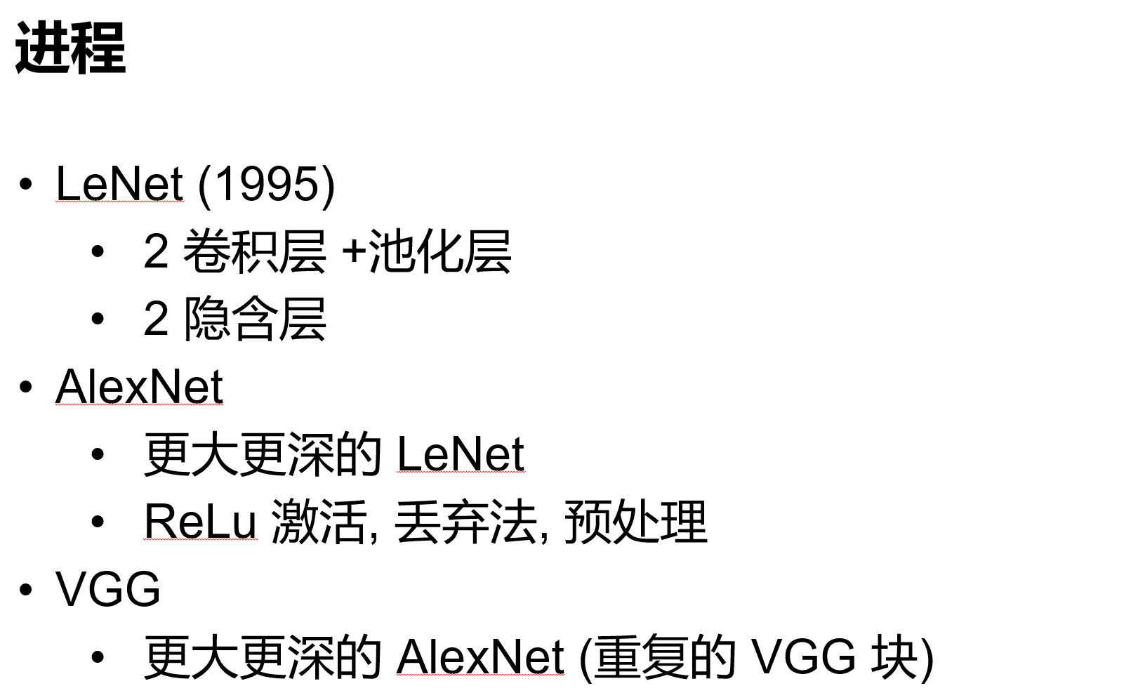
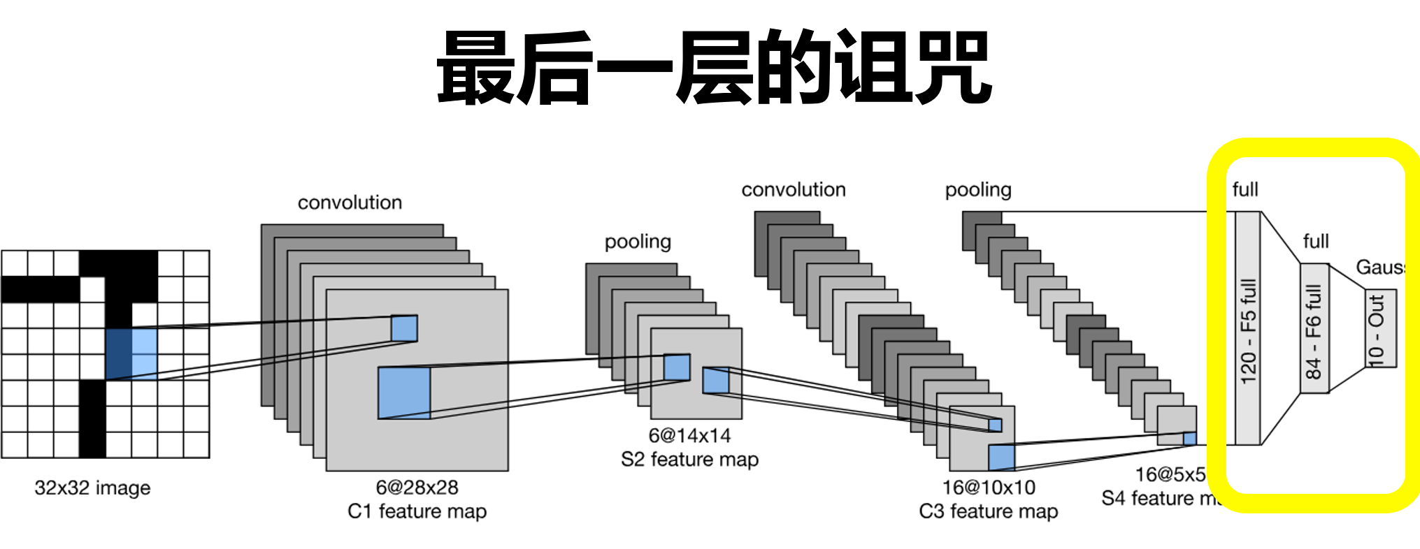
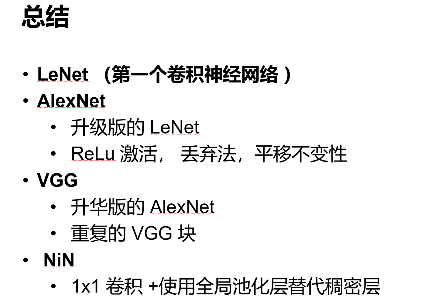
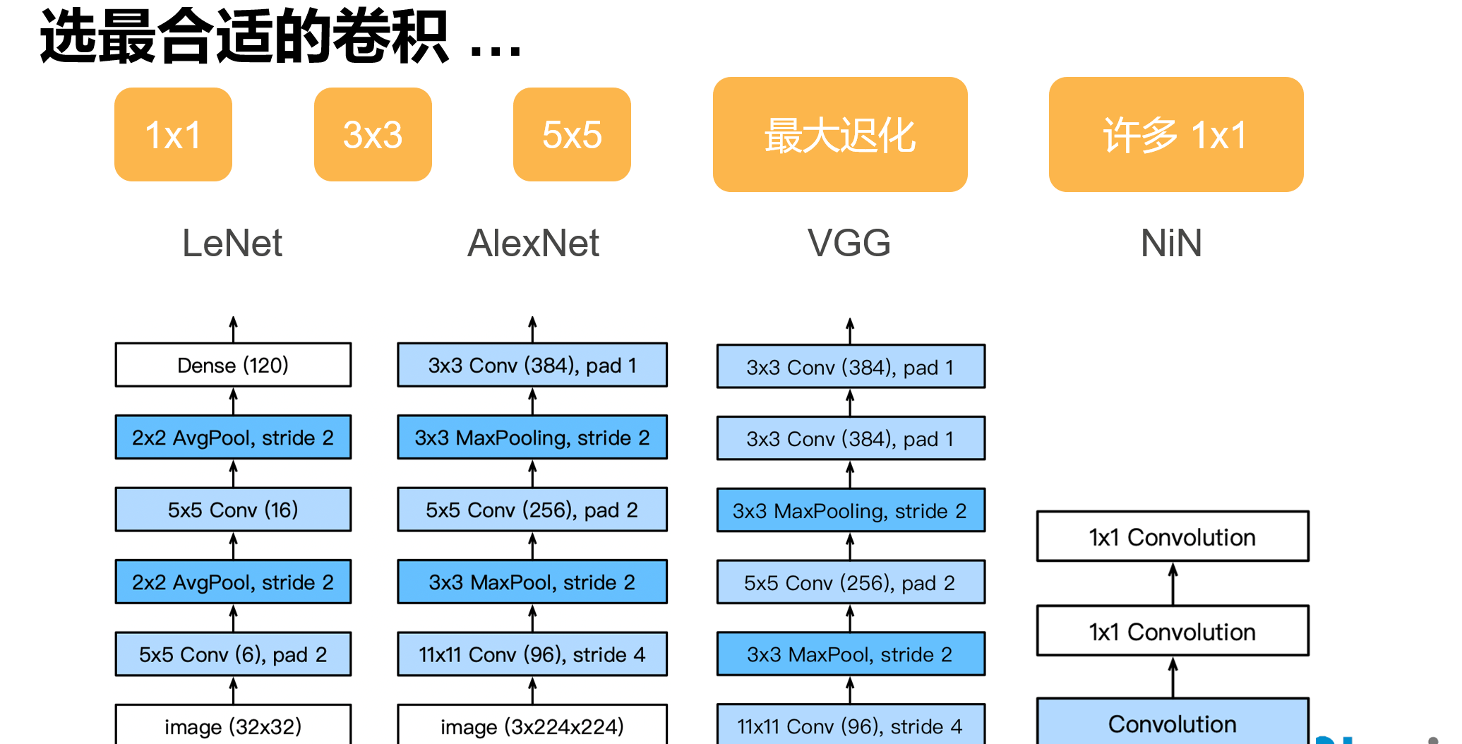
经典卷积神经网络 LeNet
虽然现在看来有一些东西已经过时了,但是它的出现证实了卷积神经网络在图片处理中确实大有益处,且启发了后来了AlexNet
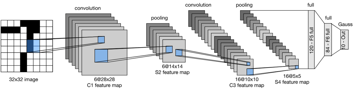
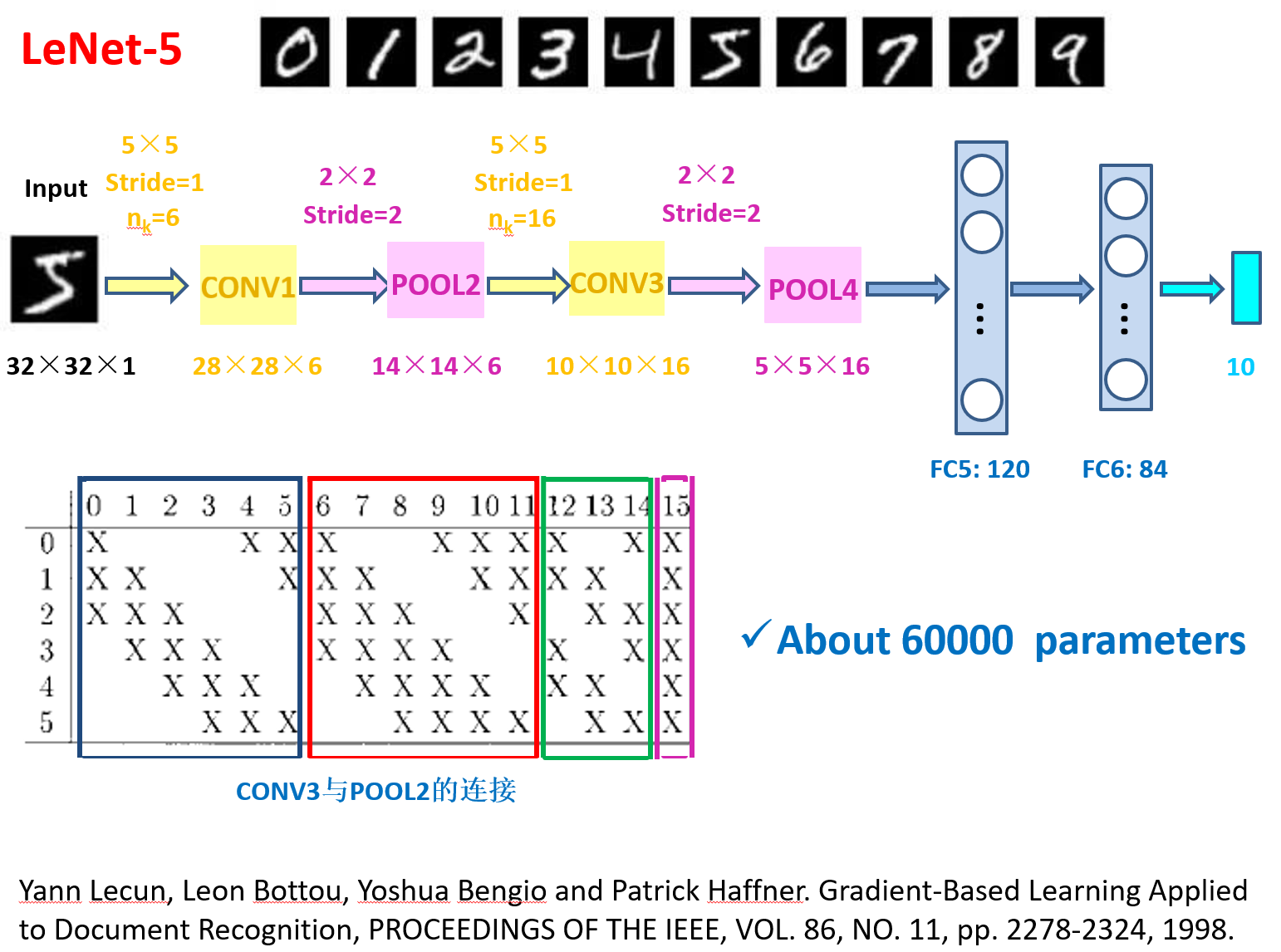
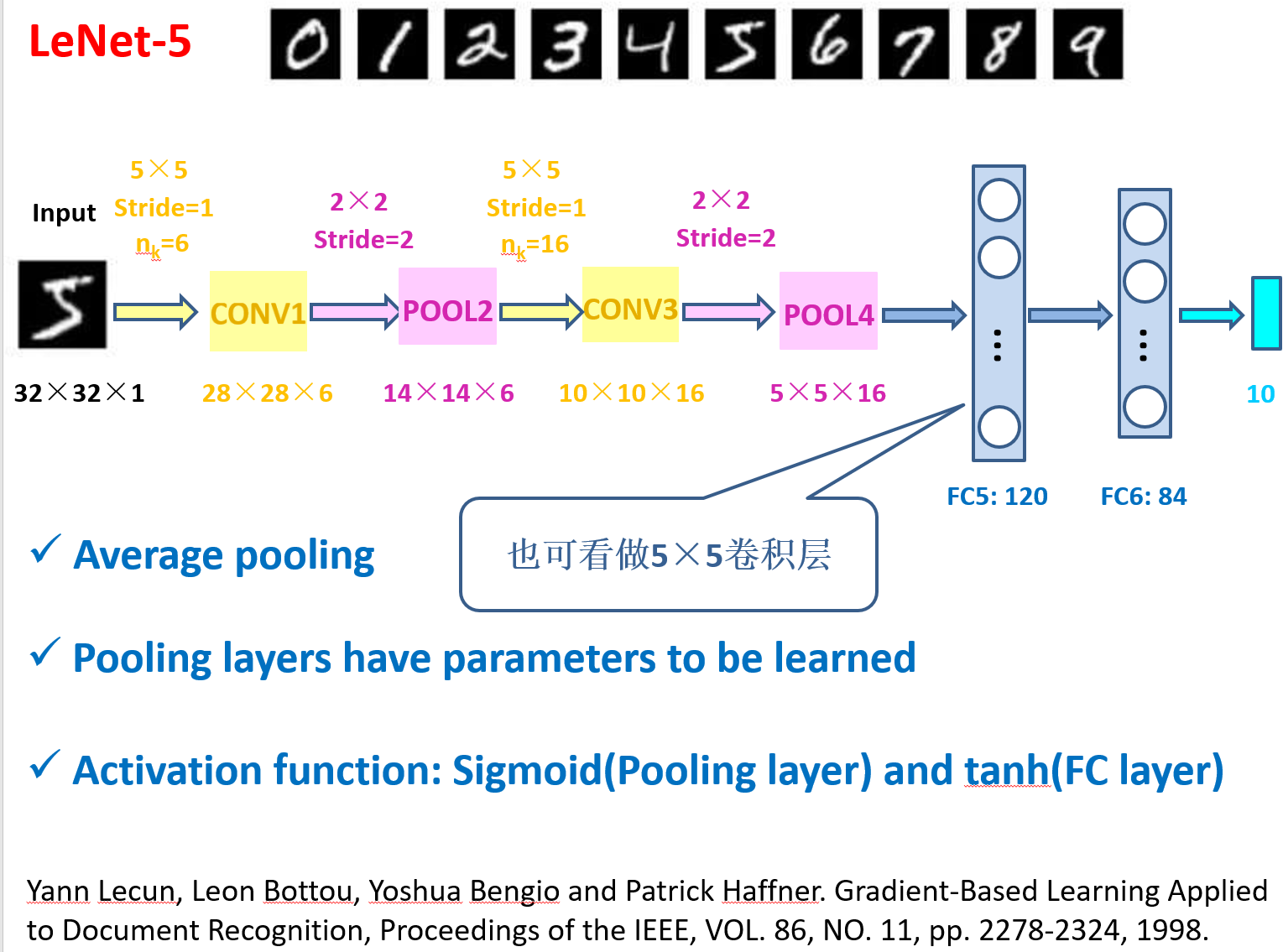
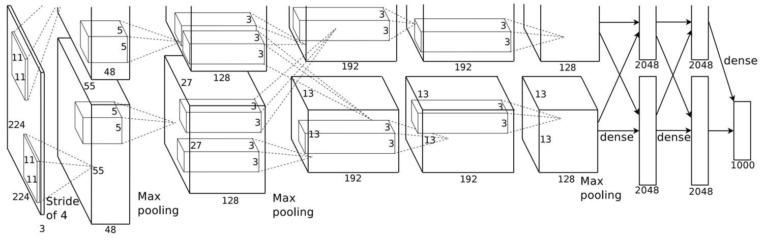
网络架构
import torch
from torch import nn
from d2l import torch as d2l

net = nn.Sequential(
    nn.Conv2d(1, 6, kernel_size=5, padding=2), nn.Sigmoid(),
    nn.AvgPool2d(kernel_size=2, stride=2),
    nn.Conv2d(6, 16, kernel_size=5), nn.Sigmoid(),
    nn.AvgPool2d(kernel_size=2, stride=2),
    nn.Flatten(),
    nn.Linear(16 * 5 * 5, 120), nn.Sigmoid(),
    nn.Linear(120, 84), nn.Sigmoid(),
    nn.Linear(84, 10))
检查模型
X = torch.rand(size=(1, 1, 28, 28), dtype=torch.float32)
for layer in net:
    X = layer(X)
    print(layer.__class__.__name__,'output shape: \t',X.shape)
输出:
Conv2d output shape: 	 torch.Size([1, 6, 28, 28])
Sigmoid output shape: 	 torch.Size([1, 6, 28, 28])
AvgPool2d output shape: 	 torch.Size([1, 6, 14, 14])
Conv2d output shape: 	 torch.Size([1, 16, 10, 10])
Sigmoid output shape: 	 torch.Size([1, 16, 10, 10])
AvgPool2d output shape: 	 torch.Size([1, 16, 5, 5])
Flatten output shape: 	 torch.Size([1, 400])
Linear output shape: 	 torch.Size([1, 120])
Sigmoid output shape: 	 torch.Size([1, 120])
Linear output shape: 	 torch.Size([1, 84])
Sigmoid output shape: 	 torch.Size([1, 84])
Linear output shape: 	 torch.Size([1, 10])
调参经验:
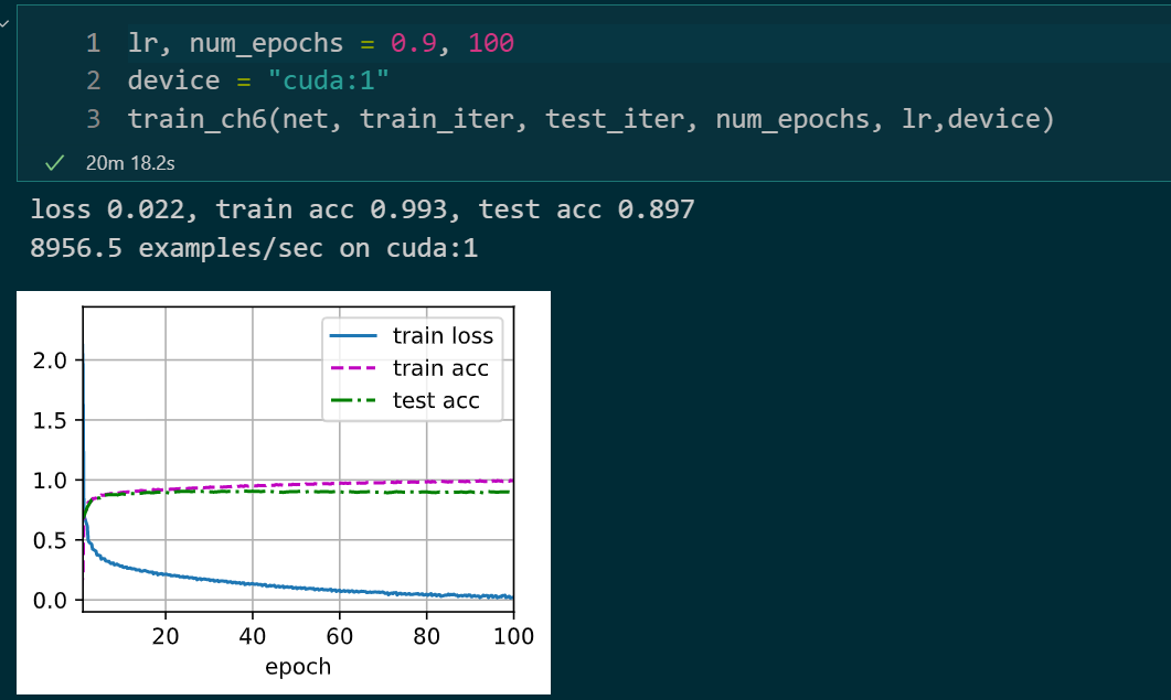
LeNet 调参记录
epochs : 100 batch_size : 256 激活函数 : Sigmoid lr : 0.9

epochs : 100 batch_size : 32 激活函数 : Sigmoid lr : 0.9
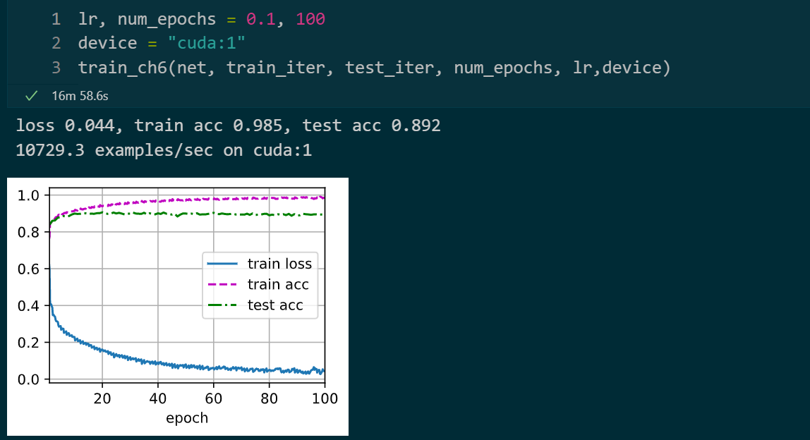
epochs : 100 batch_size : 256 激活函数 : ReLU lr : 0.1
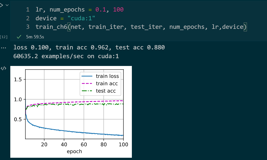
epochs : 100 batch_size : 32 激活函数 : ReLU lr : 0.1
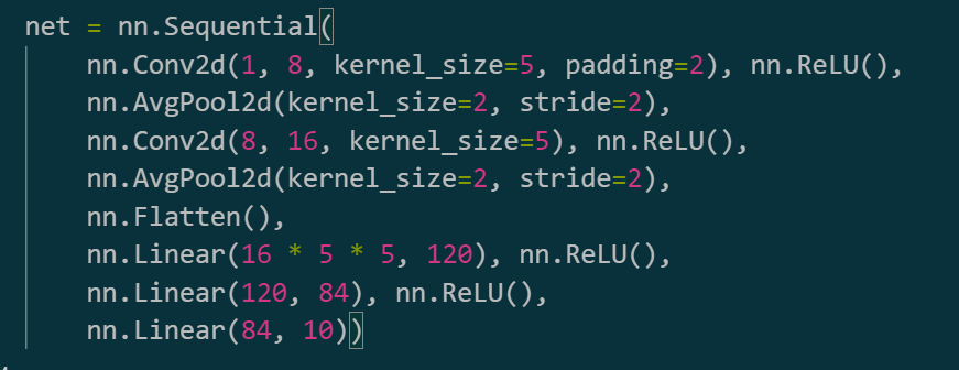
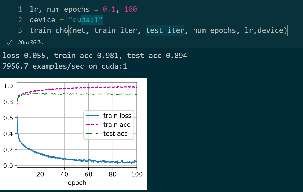
epochs : 100 batch_size : 32 激活函数 : ReLU lr : 0.1 改变通道:如下
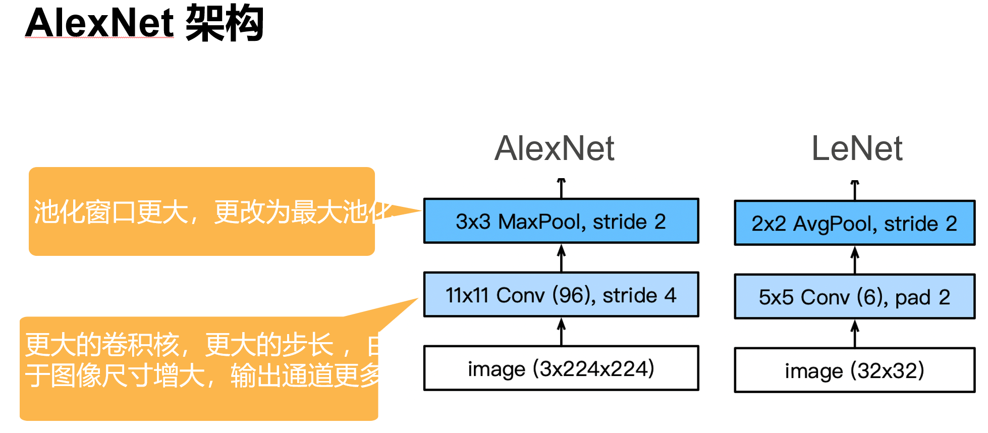
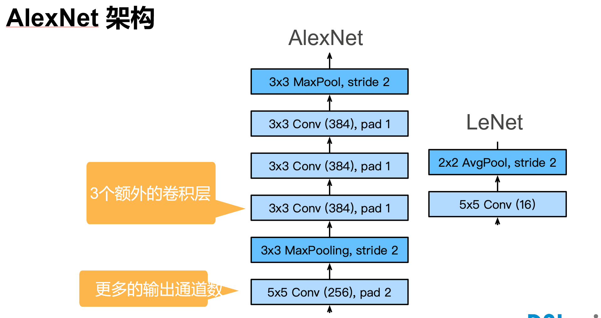
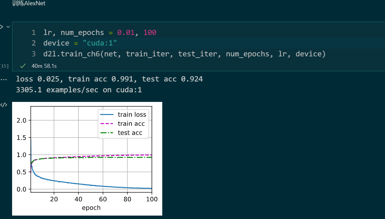
深度卷积神经网络 AlexNet
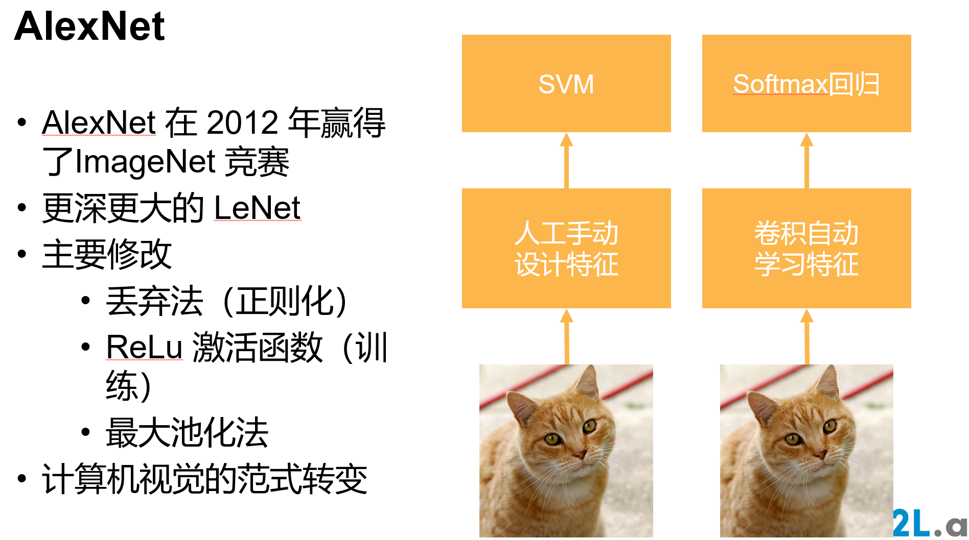
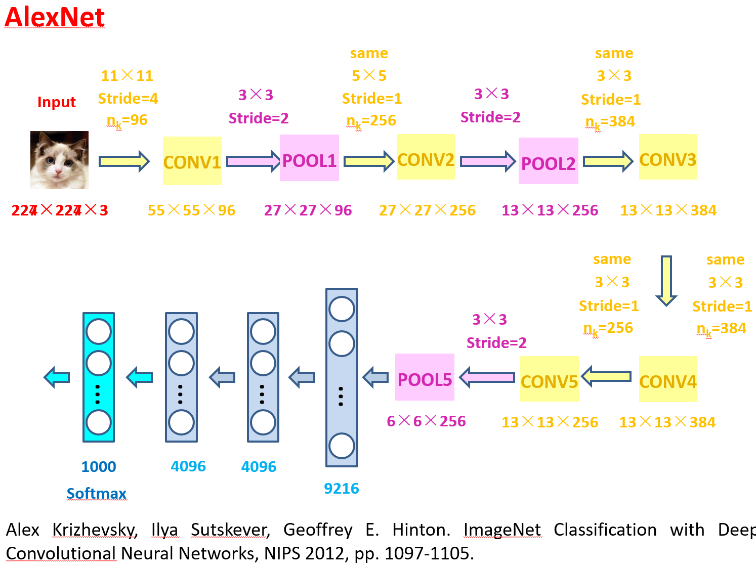
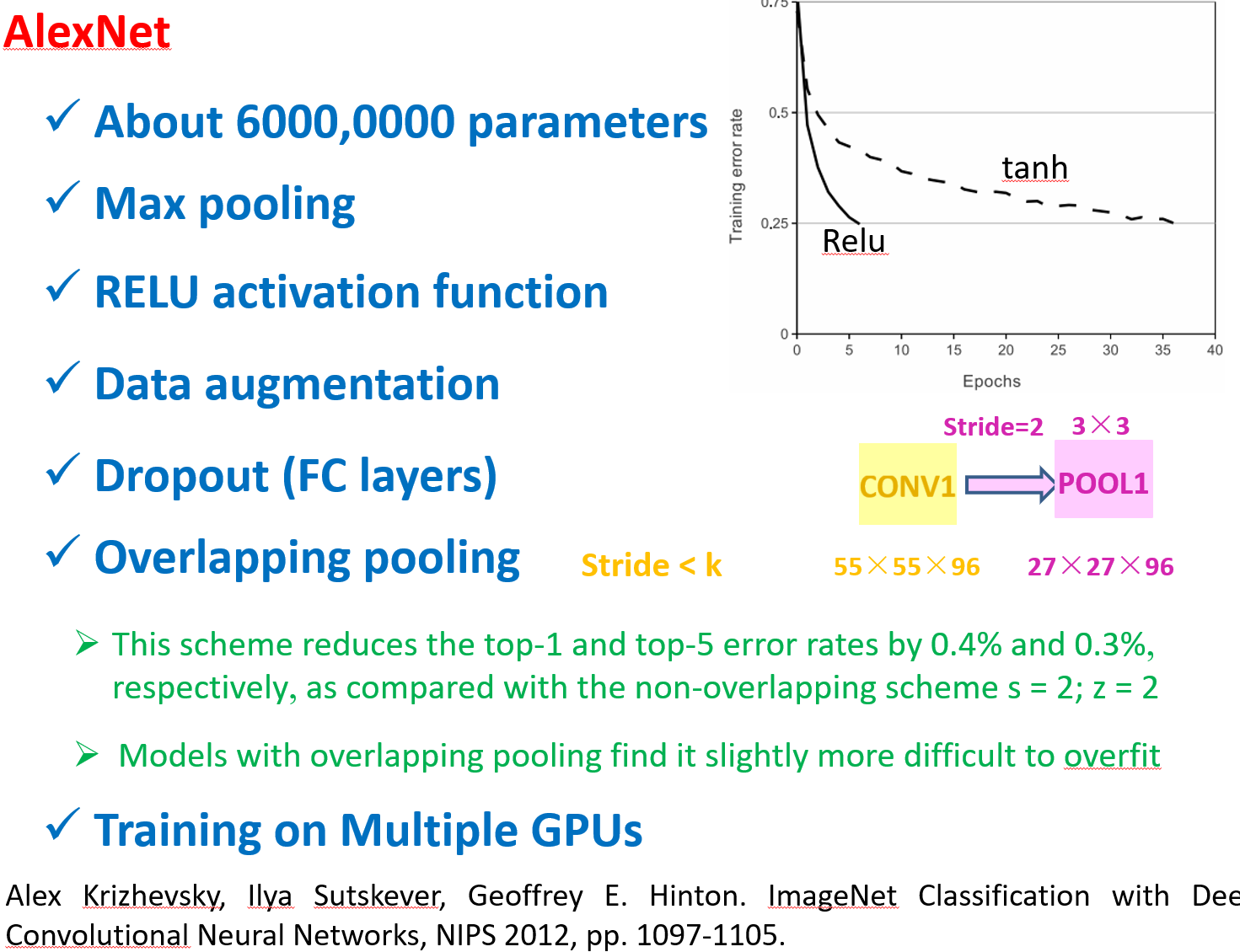
'''
根据AlexNet论文: https://papers.nips.cc/paper/2012/file/c399862d3b9d6b76c8436e924a68c45b-Paper.pdf ,实现如下:
'''
net = nn.Sequential(
      nn.Conv2d(3,96,kernel_size=11,stride=4,padding=2),nn.ReLU(),
      nn.MaxPool2d(kernel_size=3,stride=2), #
      nn.Conv2d(96,128*2,kernel_size=5,padding=2),nn.ReLU(),
      nn.MaxPool2d(kernel_size=3,stride=2),
      nn.Conv2d(128*2,192*2,kernel_size=3,padding=1),nn.ReLU(),
      nn.Conv2d(192*2,192*2,kernel_size=3,padding=1),nn.ReLU(),
      nn.Conv2d(192*2,128*2,kernel_size=3,padding=1),nn.ReLU(),
      nn.MaxPool2d(kernel_size=3,stride=2), # 6*6*256
      nn.Flatten(),
      nn.Linear(6*6*256,2048*2),nn.ReLU(),nn.Dropout(p=0.5),
      nn.Linear(2048*2,2048*2),nn.ReLU(),nn.Dropout(p=0.5),
      nn.Linear(2048*2,1000),nn.ReLU(),
    )


X = torch.randn(1, 3, 224, 224)
for layer in net:
    X=layer(X)
    print(layer.__class__.__name__,'output shape:\t',X.shape)

'''
Conv2d output shape:	 torch.Size([1, 96, 55, 55])
ReLU output shape:	 torch.Size([1, 96, 55, 55])
MaxPool2d output shape:	 torch.Size([1, 96, 27, 27])
Conv2d output shape:	 torch.Size([1, 256, 27, 27])
ReLU output shape:	 torch.Size([1, 256, 27, 27])
MaxPool2d output shape:	 torch.Size([1, 256, 13, 13])
Conv2d output shape:	 torch.Size([1, 384, 13, 13])
ReLU output shape:	 torch.Size([1, 384, 13, 13])
Conv2d output shape:	 torch.Size([1, 384, 13, 13])
ReLU output shape:	 torch.Size([1, 384, 13, 13])
Conv2d output shape:	 torch.Size([1, 256, 13, 13])
ReLU output shape:	 torch.Size([1, 256, 13, 13])
MaxPool2d output shape:	 torch.Size([1, 256, 6, 6])
Flatten output shape:	 torch.Size([1, 9216])
Linear output shape:	 torch.Size([1, 4096])
ReLU output shape:	 torch.Size([1, 4096])
Dropout output shape:	 torch.Size([1, 4096])
Linear output shape:	 torch.Size([1, 4096])
ReLU output shape:	 torch.Size([1, 4096])
Dropout output shape:	 torch.Size([1, 4096])
Linear output shape:	 torch.Size([1, 1000])
ReLU output shape:	 torch.Size([1, 1000])
'''
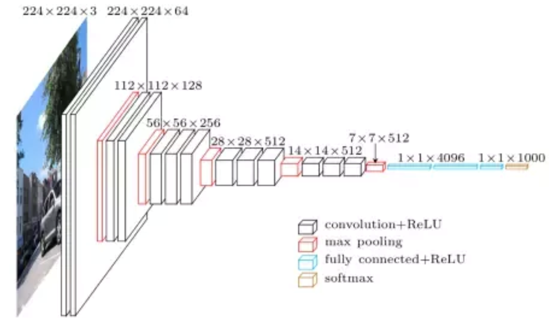
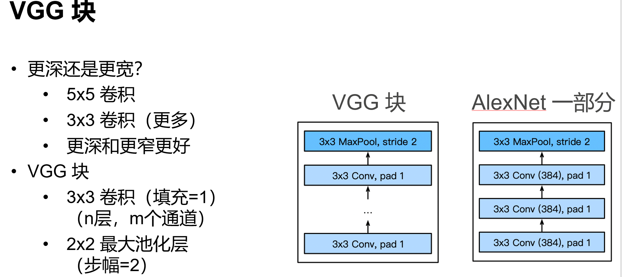
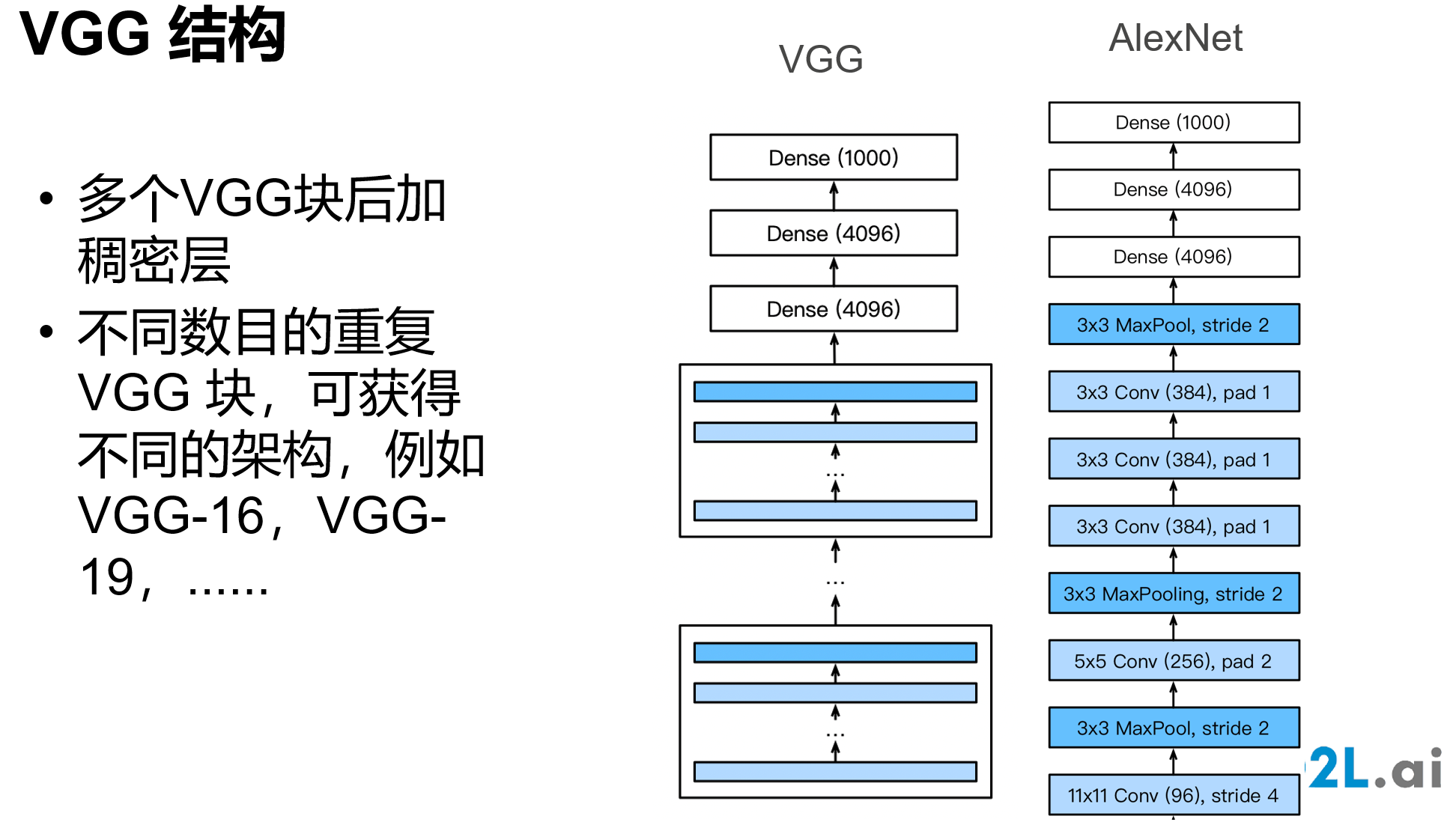
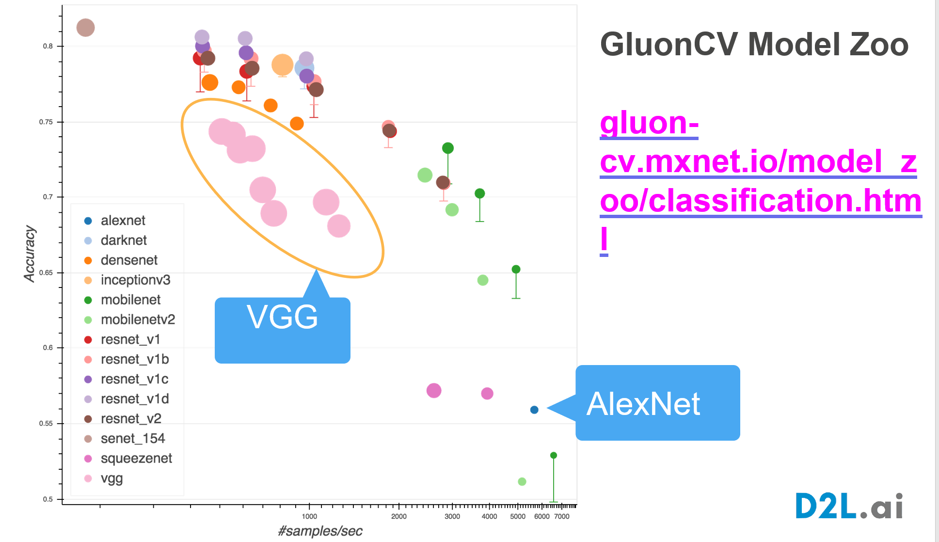
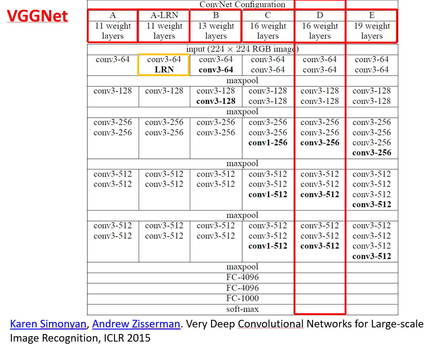
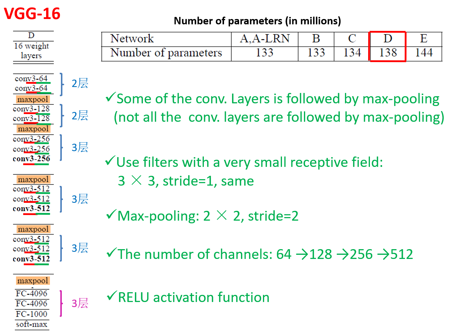
使用块的网络 VGG
VGGNet 使用VGG块,采用3x3的卷积,堆的更深
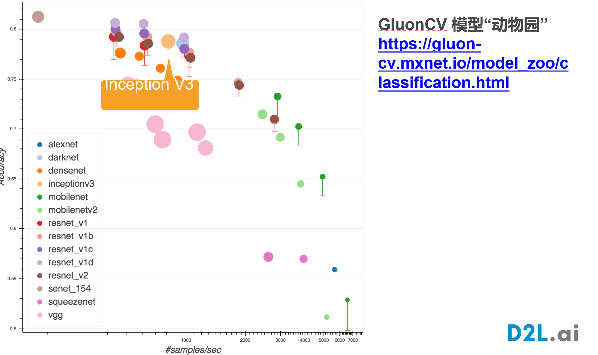
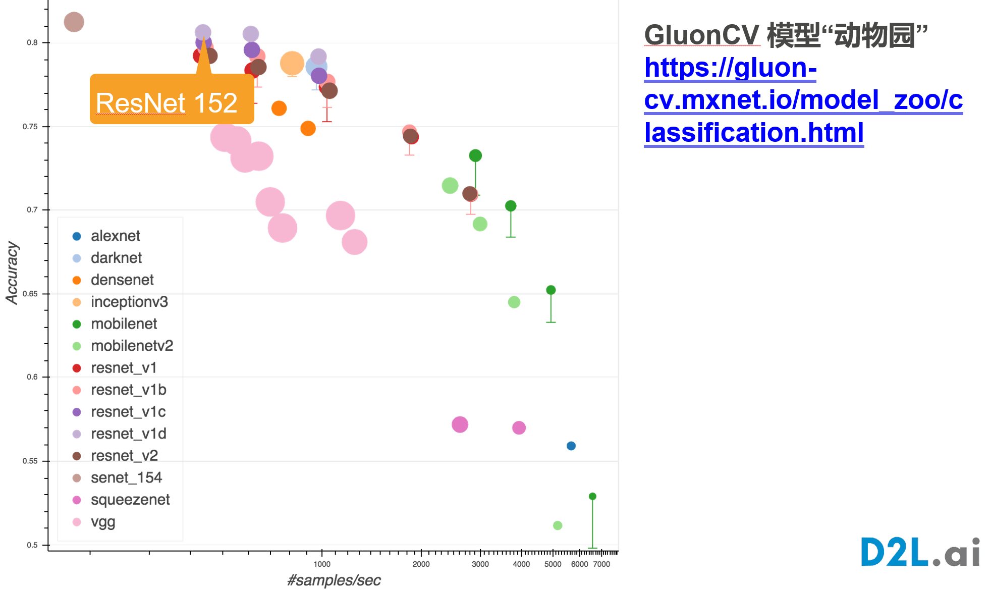
网址:https://cv.gluon.ai/model_zoo/classification.html
VGG11代码:
# vgg_net
def vgg_block(num_convs, in_channels, out_channels):
layers = []
for _ in range(num_convs):
layers.append(nn.Conv2d(in_channels, out_channels,
kernel_size=3, padding=1))
layers.append(nn.ReLU())
in_channels = out_channels
layers.append(nn.MaxPool2d(kernel_size=2,stride=2))
return nn.Sequential(*layers)
class VGGNet11(nn.Module):
def __init__(self,conv_arch:tuple,in_channels) -> None:
super(VGGNet11,self).__init__()
layers: List[nn.Module] = []
for num_conv,out_channels in conv_arch:
layers.append(vgg_block(num_conv,in_channels,out_channels))
in_channels = out_channels
self.model = nn.Sequential(*layers,
nn.Flatten(),
nn.Linear(in_channels * 7 * 7,4096),nn.ReLU(),nn.Dropout(p=0.5),
nn.Linear(4096,4096),nn.ReLU(),nn.Dropout(p=0.5),
nn.Linear(4096,176),
)
def forward(self,x):
return self.model(x)
def checkout_channel(self,X=None):
for blk in self.model:
X = blk(X)
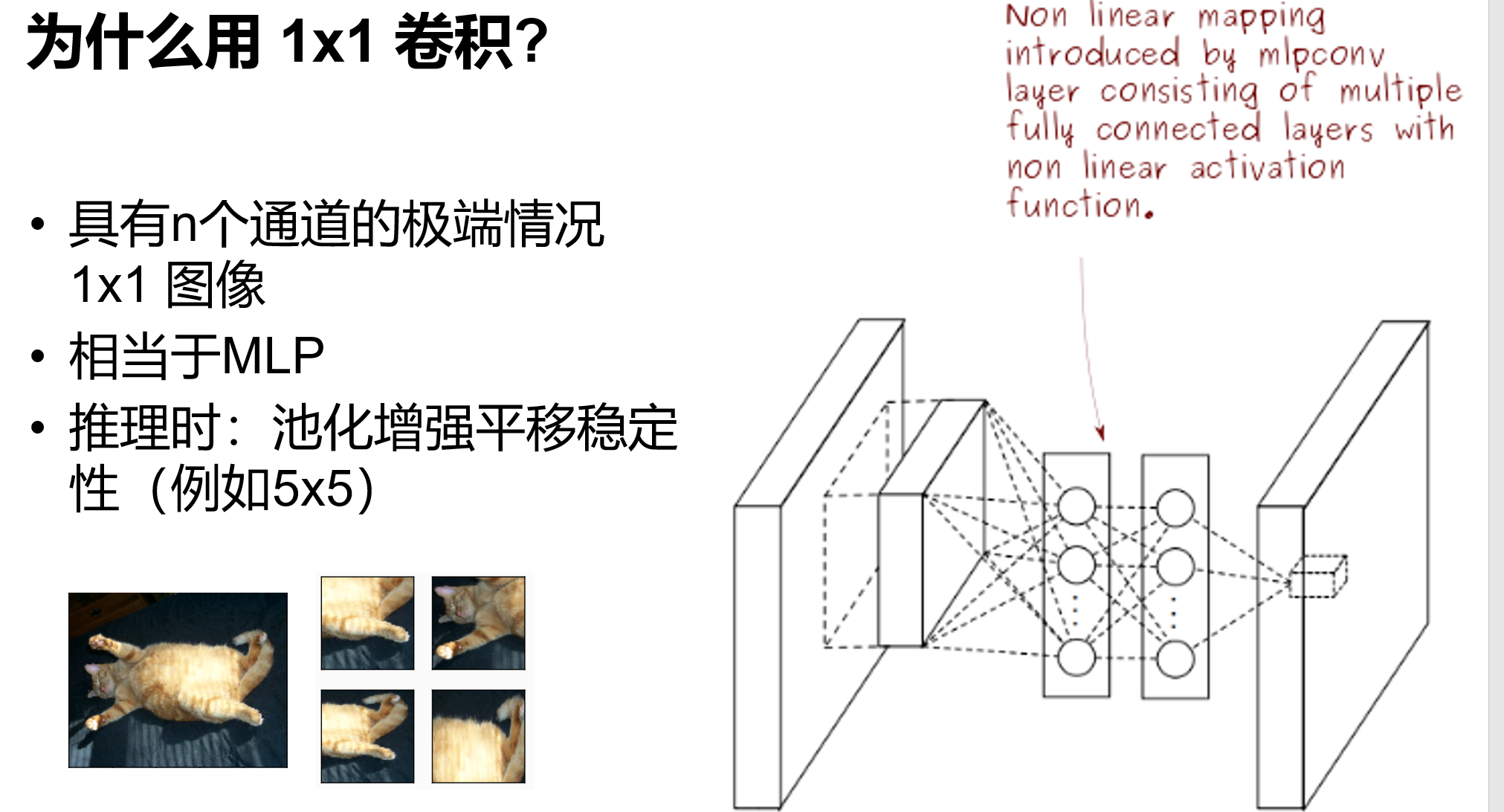
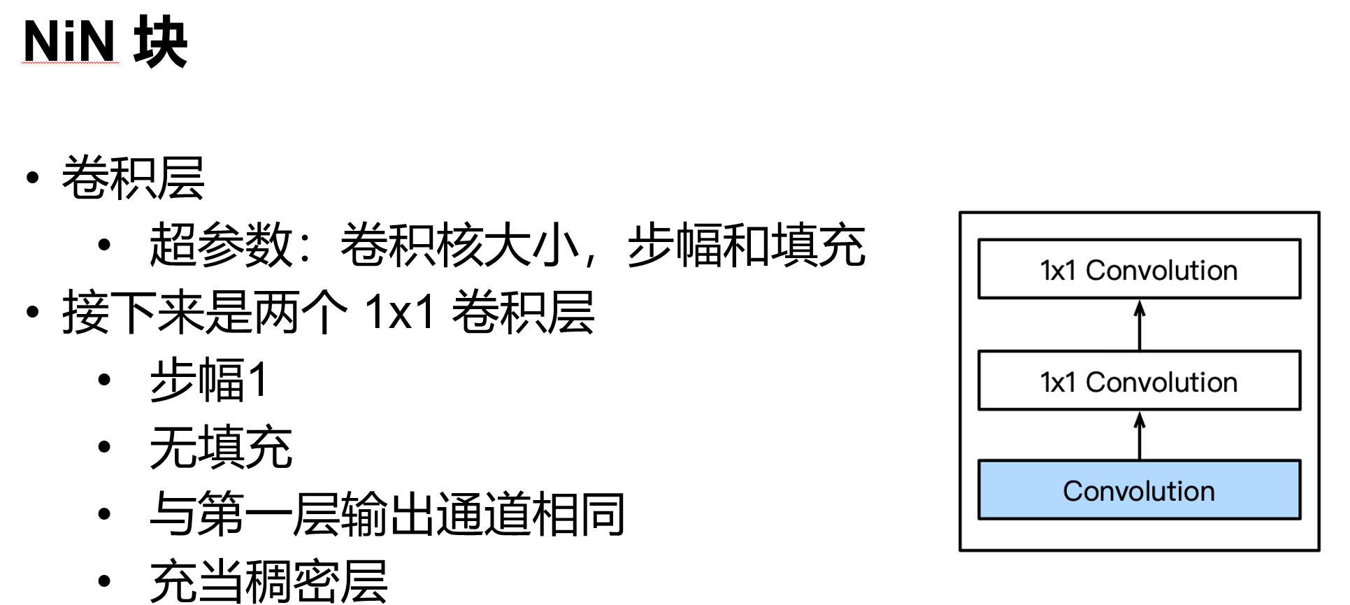
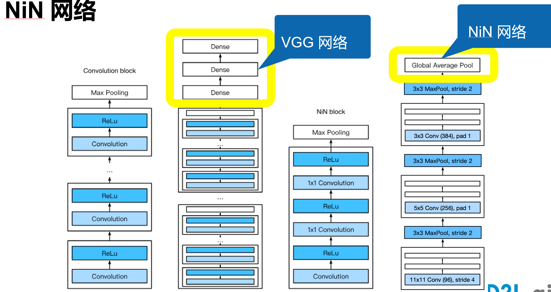
print(blk.__class__.__name__,'output shape:\t',X.shape)网络中的网络 NiN
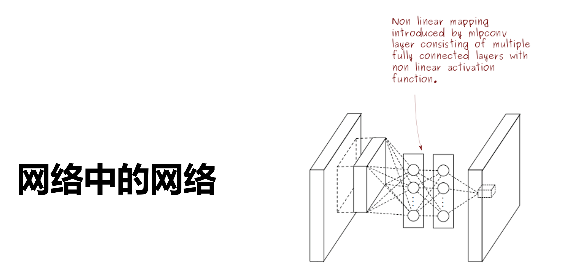
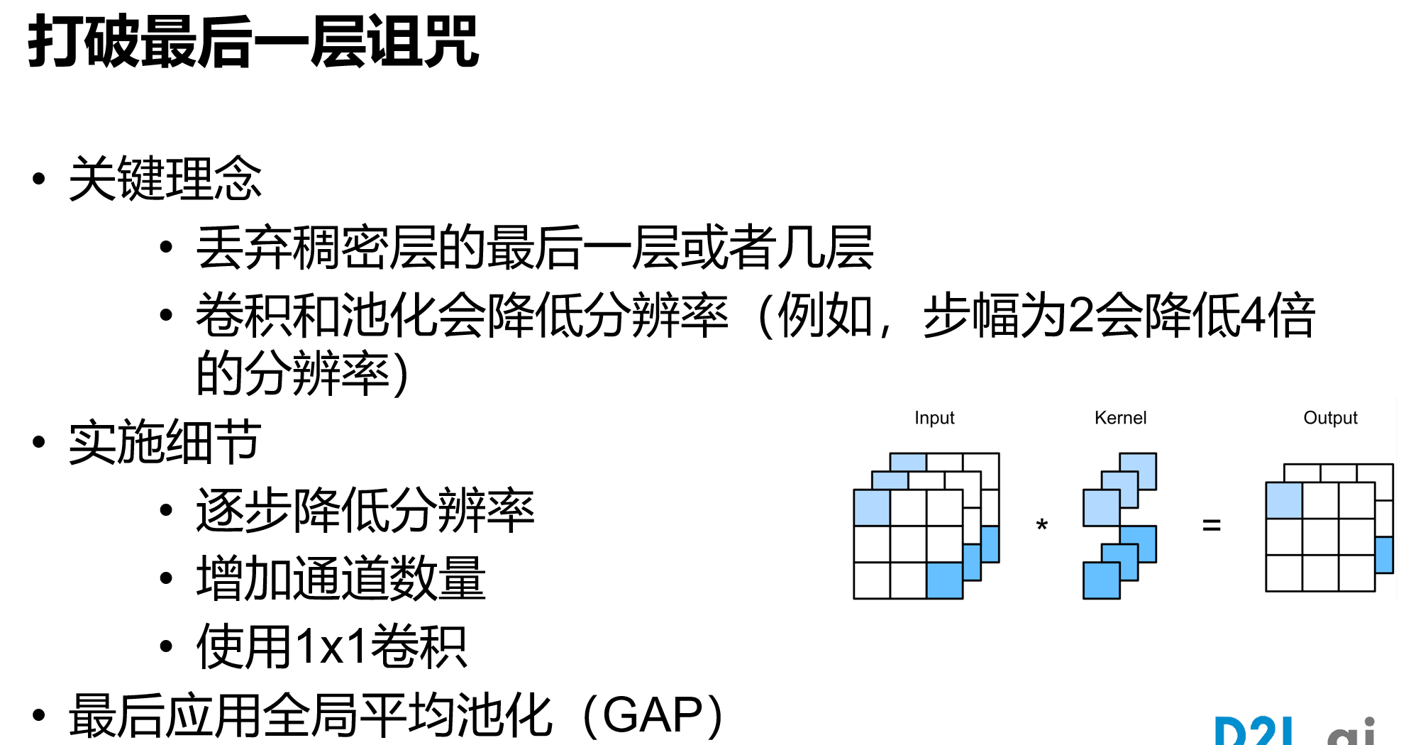
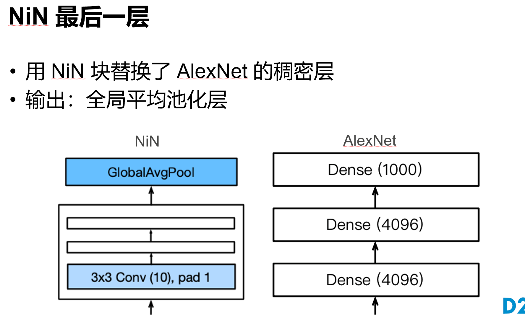
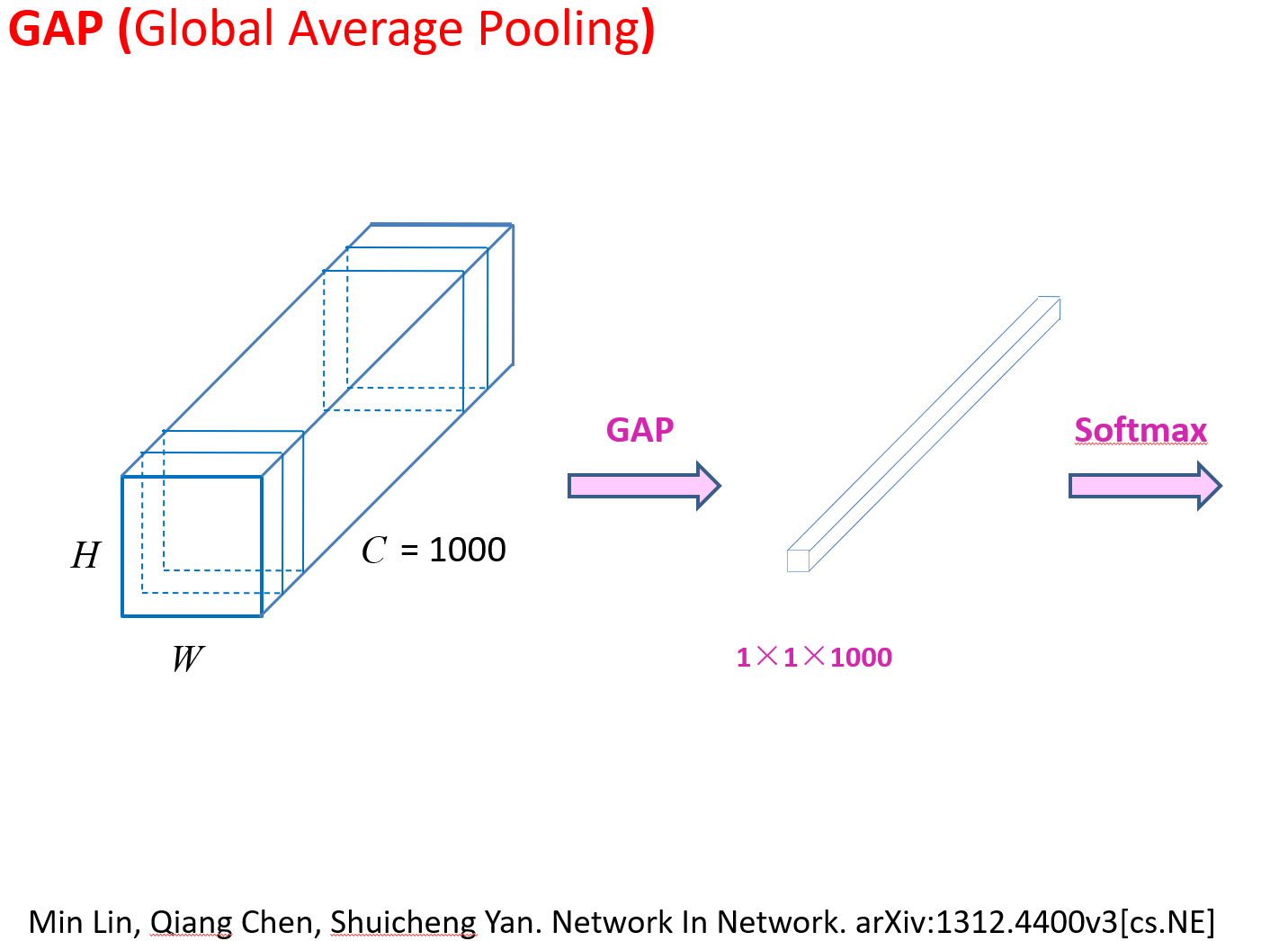
文章中说:与全连接层相比,global average pooling (GAP) 的两个优点:
① One advantage of global average pooling over the fully connected layers is that it is more native to the convolution structure by enforcing correspondences between feature maps and categories. (GAP 通过强制使特征图和类别之间相对应,对于卷积结构更来说这个转换更自然。)
② Another advantage is that there is no parameter to optimize in the global average pooling thus overfitting is avoided at this layer. (GAP 层没有参数用于优化,避免了过拟合。)
def nin_block(in_channels, out_channels, kernel_size, strides, padding):
return nn.Sequential(
nn.Conv2d(in_channels, out_channels, kernel_size, strides, padding),
nn.ReLU(),
nn.Conv2d(out_channels, out_channels, kernel_size=1), nn.ReLU(),
nn.Conv2d(out_channels, out_channels, kernel_size=1), nn.ReLU())
net = nn.Sequential(
nin_block(1, 96, kernel_size=11, strides=4, padding=0),
nn.MaxPool2d(3, stride=2),
nin_block(96, 256, kernel_size=5, strides=1, padding=2),
nn.MaxPool2d(3, stride=2),
nin_block(256, 384, kernel_size=3, strides=1, padding=1),
nn.MaxPool2d(3, stride=2),
nn.Dropout(0.5),
nin_block(384, 10, kernel_size=3, strides=1, padding=1),
nn.AdaptiveAvgPool2d((1, 1)),
nn.Flatten())
X = torch.rand(size=(1, 1, 224, 224))
for layer in net:
X = layer(X)
print(layer.__class__.__name__,'output shape:\t', X.shape)
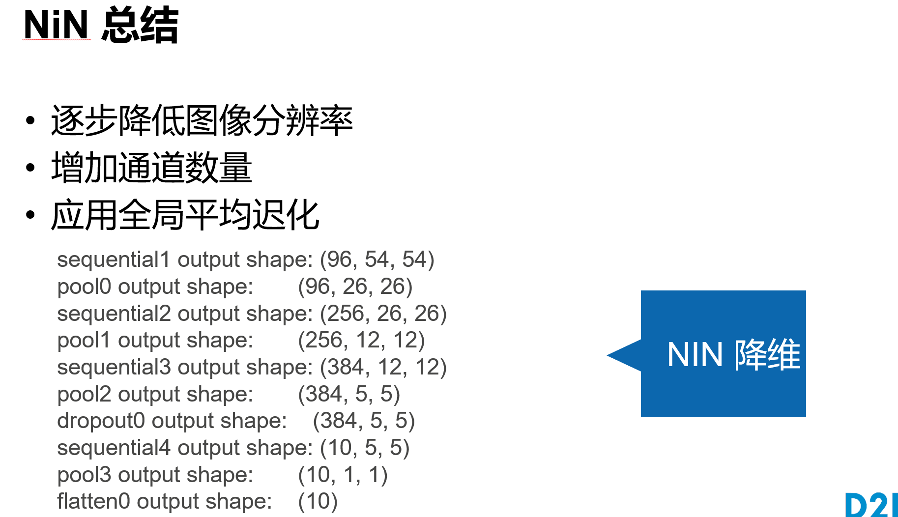
'''
Sequential output shape: torch.Size([1, 96, 54, 54])
MaxPool2d output shape: torch.Size([1, 96, 26, 26])
Sequential output shape: torch.Size([1, 256, 26, 26])
MaxPool2d output shape: torch.Size([1, 256, 12, 12])
Sequential output shape: torch.Size([1, 384, 12, 12])
MaxPool2d output shape: torch.Size([1, 384, 5, 5])
Dropout output shape: torch.Size([1, 384, 5, 5])
Sequential output shape: torch.Size([1, 10, 5, 5])
AdaptiveAvgPool2d output shape: torch.Size([1, 10, 1, 1])
Flatten output shape: torch.Size([1, 10])
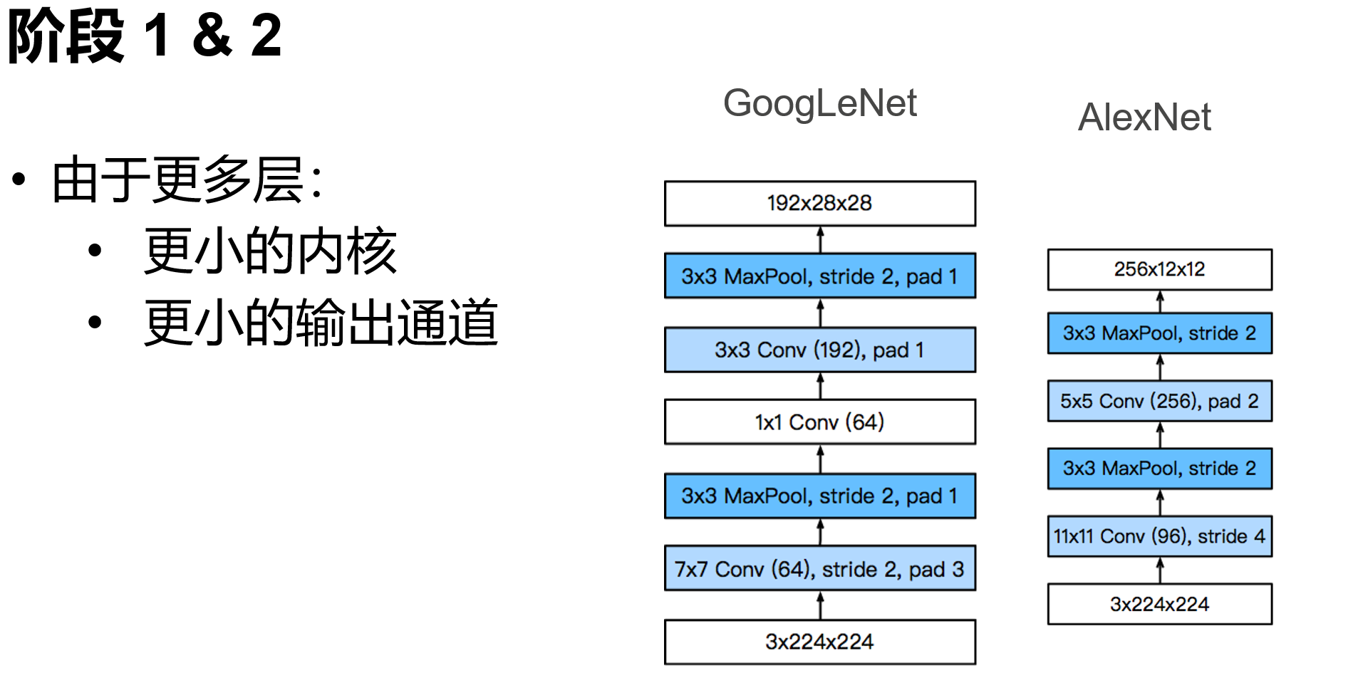
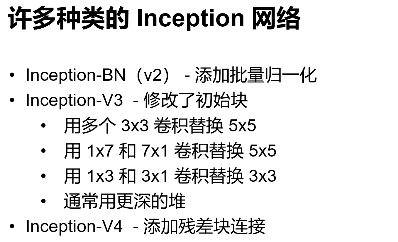
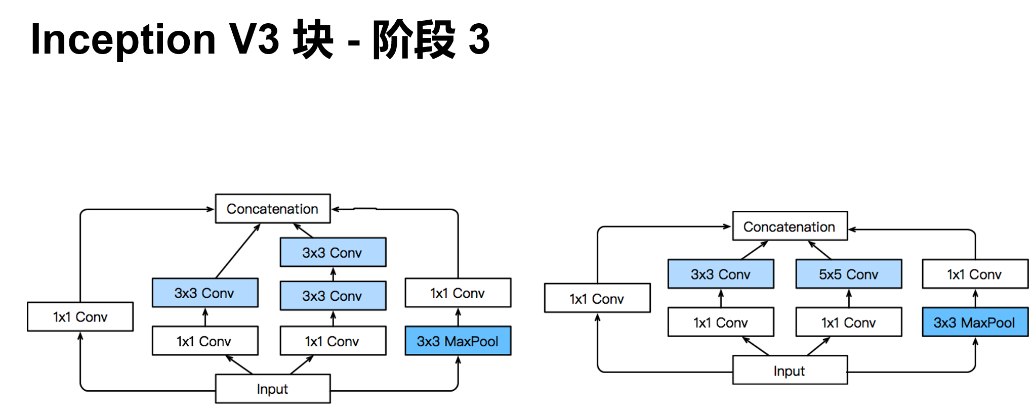
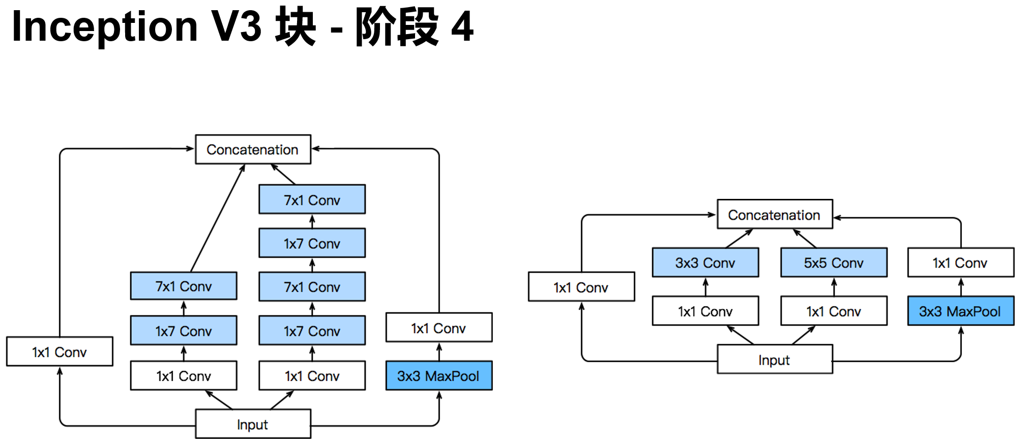
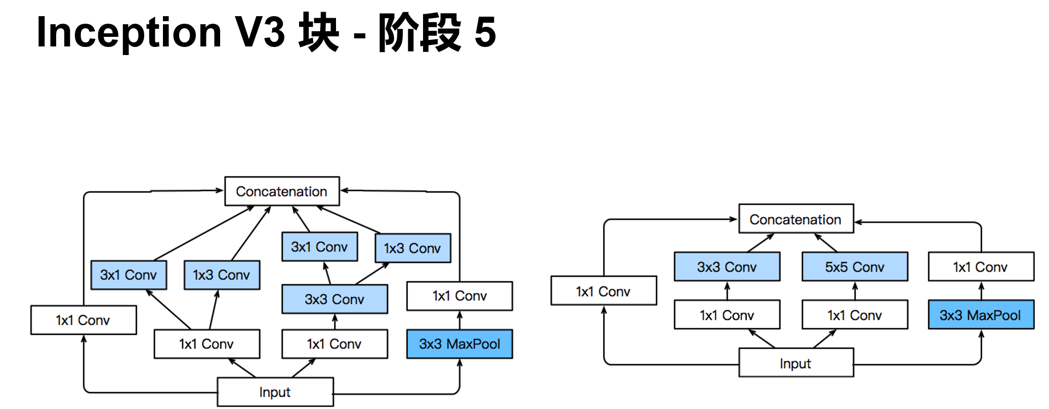
'''含并行连结的网络 GoogLeNet / Inception V3
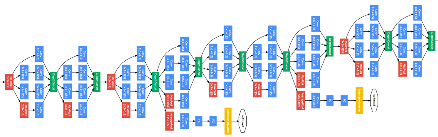
干嘛选呢?都用就是了。
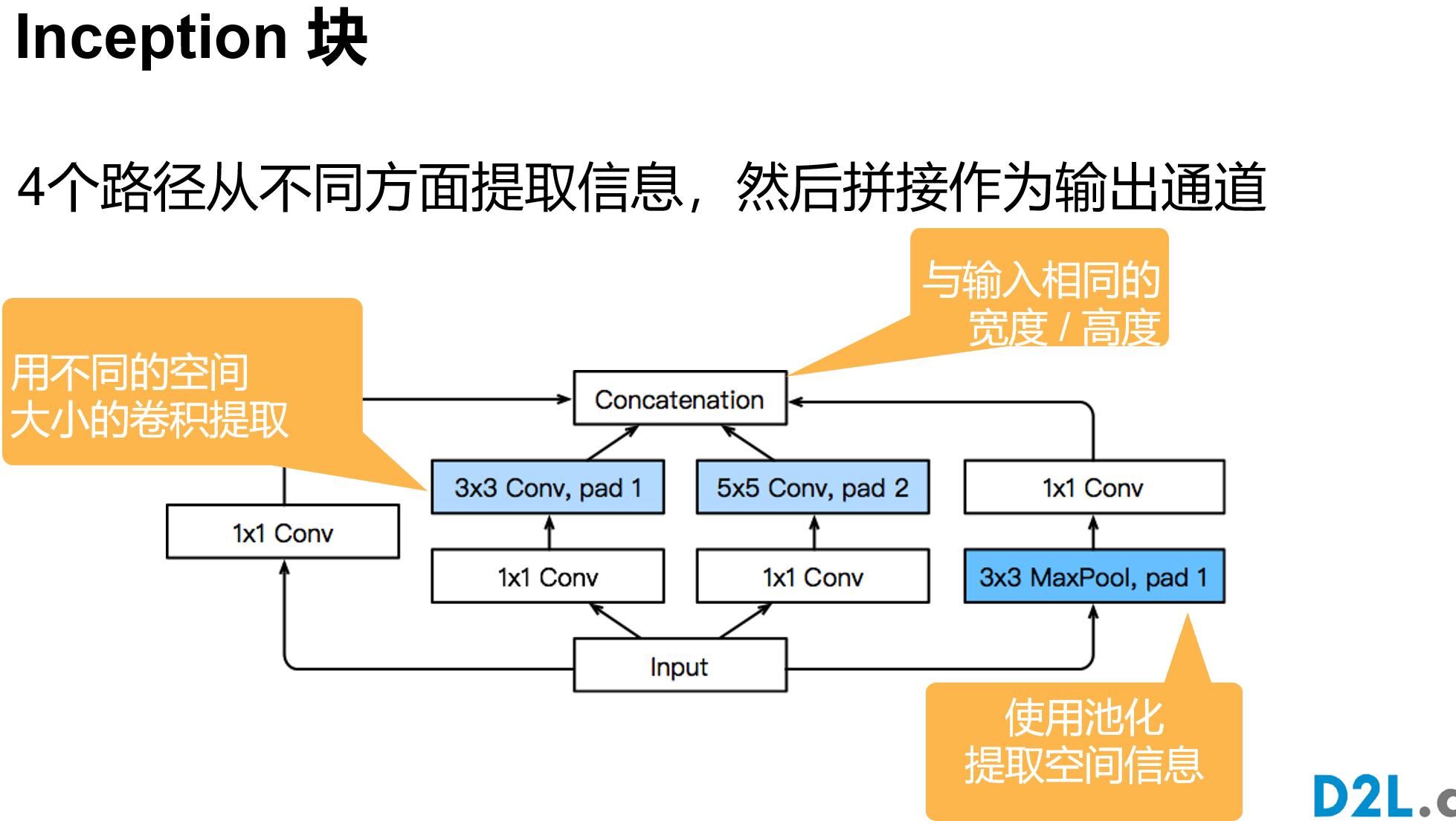
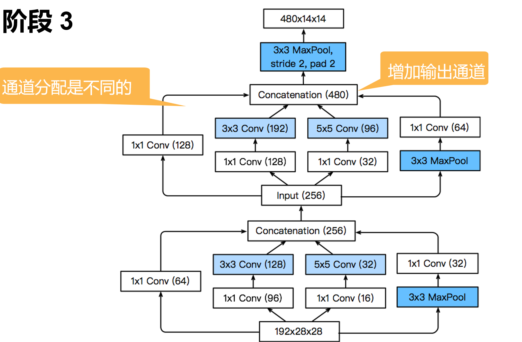
class Inception(nn.Module):
def __init__(self, in_channels, c1, c2, c3, c4, **kwargs):
super(Inception, self).__init__(**kwargs)
self.p1_1 = nn.Conv2d(in_channels, c1, kernel_size=1)
self.p2_1 = nn.Conv2d(in_channels, c2[0], kernel_size=1)
self.p2_2 = nn.Conv2d(c2[0], c2[1], kernel_size=3, padding=1)
self.p3_1 = nn.Conv2d(in_channels, c3[0], kernel_size=1)
self.p3_2 = nn.Conv2d(c3[0], c3[1], kernel_size=5, padding=2)
self.p4_1 = nn.MaxPool2d(kernel_size=3, stride=1, padding=1)
self.p4_2 = nn.Conv2d(in_channels, c4, kernel_size=1)
def forward(self, x):
p1 = F.relu(self.p1_1(x))
p2 = F.relu(self.p2_2(F.relu(self.p2_1(x))))
p3 = F.relu(self.p3_2(F.relu(self.p3_1(x))))
p4 = F.relu(self.p4_2(self.p4_1(x)))
return torch.cat((p1, p2, p3, p4), dim=1)
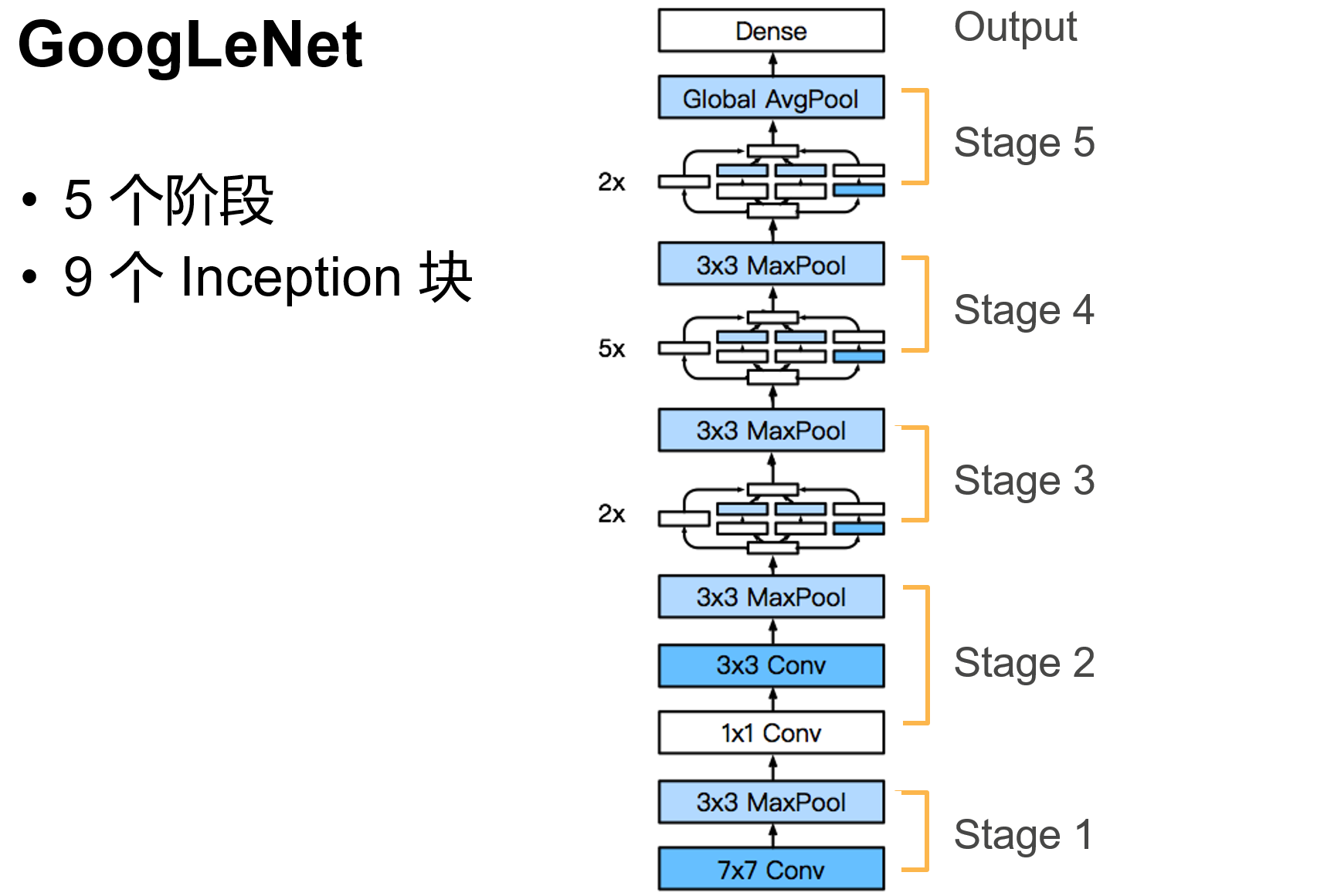
#GoogleNet 模型实现
b1 = nn.Sequential(nn.Conv2d(1, 64, kernel_size=7, stride=2, padding=3),
nn.ReLU(),
nn.MaxPool2d(kernel_size=3, stride=2, padding=1))
b2 = nn.Sequential(nn.Conv2d(64, 64, kernel_size=1),
nn.ReLU(),
nn.Conv2d(64, 192, kernel_size=3, padding=1),
nn.ReLU(),
nn.MaxPool2d(kernel_size=3, stride=2, padding=1))
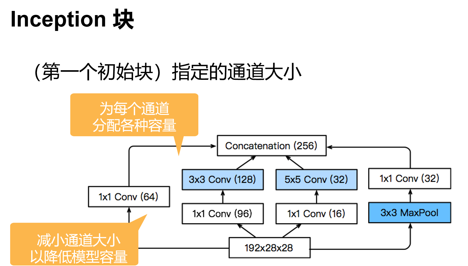
b3 = nn.Sequential(Inception(192, 64, (96, 128), (16, 32), 32),
Inception(256, 128, (128, 192), (32, 96), 64),
nn.MaxPool2d(kernel_size=3, stride=2, padding=1))
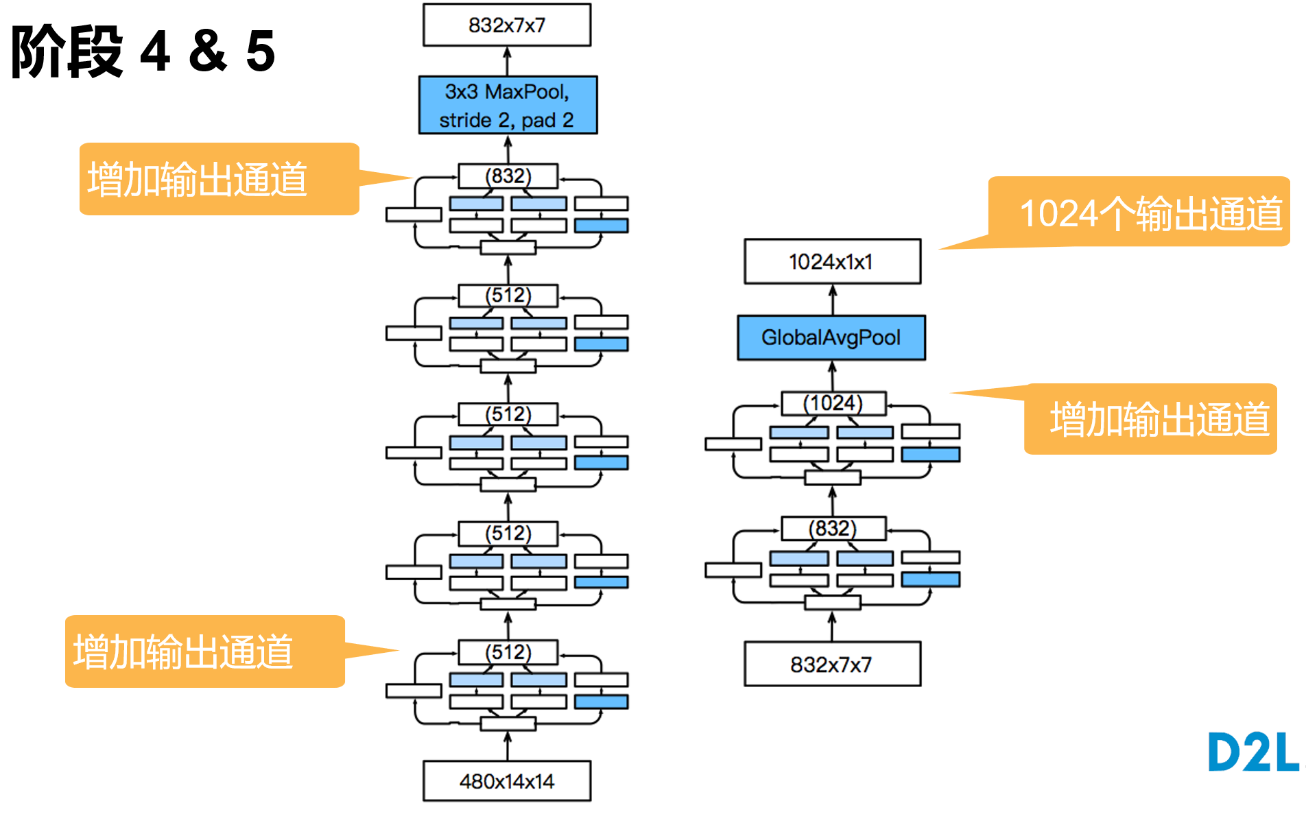
b4 = nn.Sequential(Inception(480, 192, (96, 208), (16, 48), 64),
Inception(512, 160, (112, 224), (24, 64), 64),
Inception(512, 128, (128, 256), (24, 64), 64),
Inception(512, 112, (144, 288), (32, 64), 64),
Inception(528, 256, (160, 320), (32, 128), 128),
nn.MaxPool2d(kernel_size=3, stride=2, padding=1))
b5 = nn.Sequential(Inception(832, 256, (160, 320), (32, 128), 128),
Inception(832, 384, (192, 384), (48, 128), 128),
nn.AdaptiveAvgPool2d((1,1)),
nn.Flatten())
net = nn.Sequential(b1, b2, b3, b4, b5, nn.Linear(1024, 10))
X = torch.rand(size=(1, 1, 96, 96))
for layer in net:
X = layer(X)
print(layer.__class__.__name__,'output shape:\t', X.shape)
'''
Sequential output shape: torch.Size([1, 64, 24, 24])
Sequential output shape: torch.Size([1, 192, 12, 12])
Sequential output shape: torch.Size([1, 480, 6, 6])
Sequential output shape: torch.Size([1, 832, 3, 3])
Sequential output shape: torch.Size([1, 1024])
Linear output shape: torch.Size([1, 10])
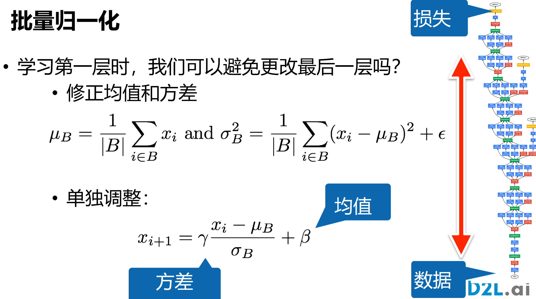
'''批量归一化
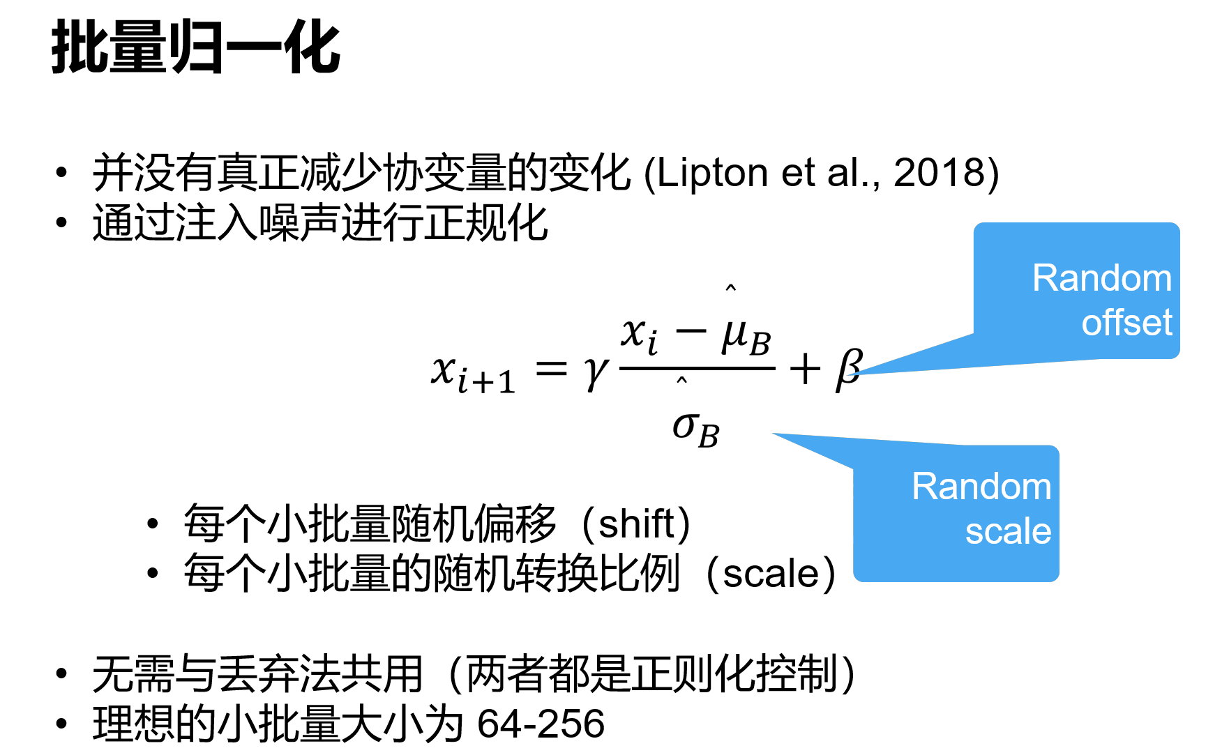
保证层间输出和梯度符合某一特定分布,以提高数据和损失的稳定性
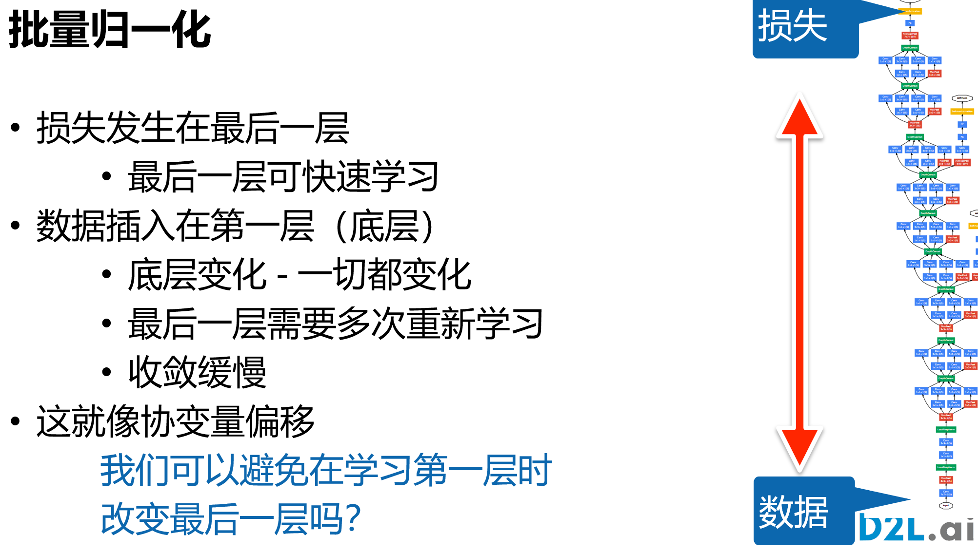
有的论文说BN并不会减少协变量偏移,只是可能加入了噪音
# start from scratch
def batch_norm(X, gamma, beta, moving_mean, moving_var, eps, momentum):
if not torch.is_grad_enabled():
X_hat = (X - moving_mean) / torch.sqrt(moving_var + eps)
else:
assert len(X.shape) in (2, 4)
if len(X.shape) == 2:
mean = X.mean(dim=0)
var = ((X - mean) ** 2).mean(dim=0)
else:
mean = X.mean(dim=(0, 2, 3), keepdim=True)
var = ((X - mean) ** 2).mean(dim=(0, 2, 3), keepdim=True)
X_hat = (X - mean) / torch.sqrt(var + eps)
moving_mean = momentum * moving_mean + (1.0 - momentum) * mean
moving_var = momentum * moving_var + (1.0 - momentum) * var
Y = gamma * X_hat + beta
return Y, moving_mean.data, moving_var.data
class BatchNorm(nn.Module):
def __init__(self, num_features, num_dims):
super().__init__()
if num_dims == 2:
shape = (1, num_features)
else:
shape = (1, num_features, 1, 1)
self.gamma = nn.Parameter(torch.ones(shape))
self.beta = nn.Parameter(torch.zeros(shape))
self.moving_mean = torch.zeros(shape)
self.moving_var = torch.ones(shape)
def forward(self, X):
if self.moving_mean.device != X.device:
self.moving_mean = self.moving_mean.to(X.device)
self.moving_var = self.moving_var.to(X.device)
Y, self.moving_mean, self.moving_var = batch_norm(
X, self.gamma, self.beta, self.moving_mean,
self.moving_var, eps=1e-5, momentum=0.9)
return Y
net = nn.Sequential(
nn.Conv2d(1, 6, kernel_size=5), BatchNorm(6, num_dims=4), nn.Sigmoid(),
nn.AvgPool2d(kernel_size=2, stride=2),
nn.Conv2d(6, 16, kernel_size=5), BatchNorm(16, num_dims=4), nn.Sigmoid(),
nn.AvgPool2d(kernel_size=2, stride=2), nn.Flatten(),
nn.Linear(16*4*4, 120), BatchNorm(120, num_dims=2), nn.Sigmoid(),
nn.Linear(120, 84), BatchNorm(84, num_dims=2), nn.Sigmoid(),
nn.Linear(84, 10))
# concise
net = nn.Sequential(
nn.Conv2d(1, 6, kernel_size=5), nn.BatchNorm2d(6), nn.Sigmoid(),
nn.AvgPool2d(kernel_size=2, stride=2),
nn.Conv2d(6, 16, kernel_size=5), nn.BatchNorm2d(16), nn.Sigmoid(),
nn.AvgPool2d(kernel_size=2, stride=2), nn.Flatten(),
nn.Linear(256, 120), nn.BatchNorm1d(120), nn.Sigmoid(),
nn.Linear(120, 84), nn.BatchNorm1d(84), nn.Sigmoid(),
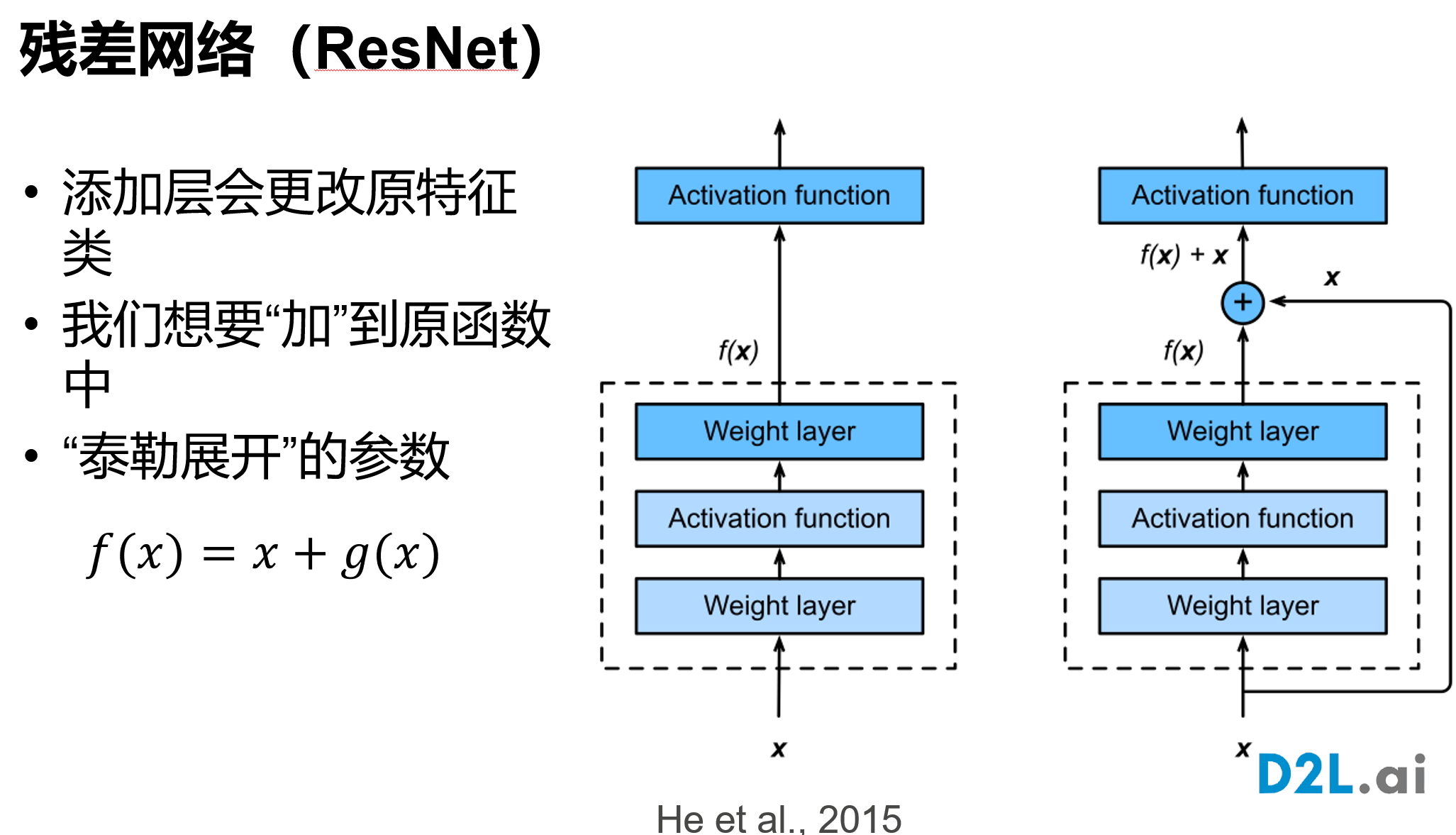
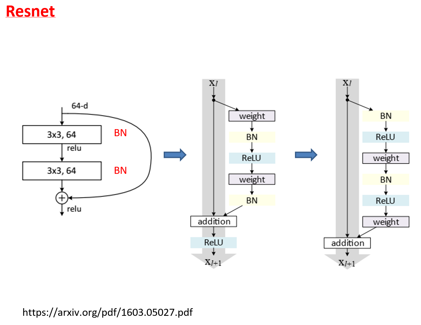
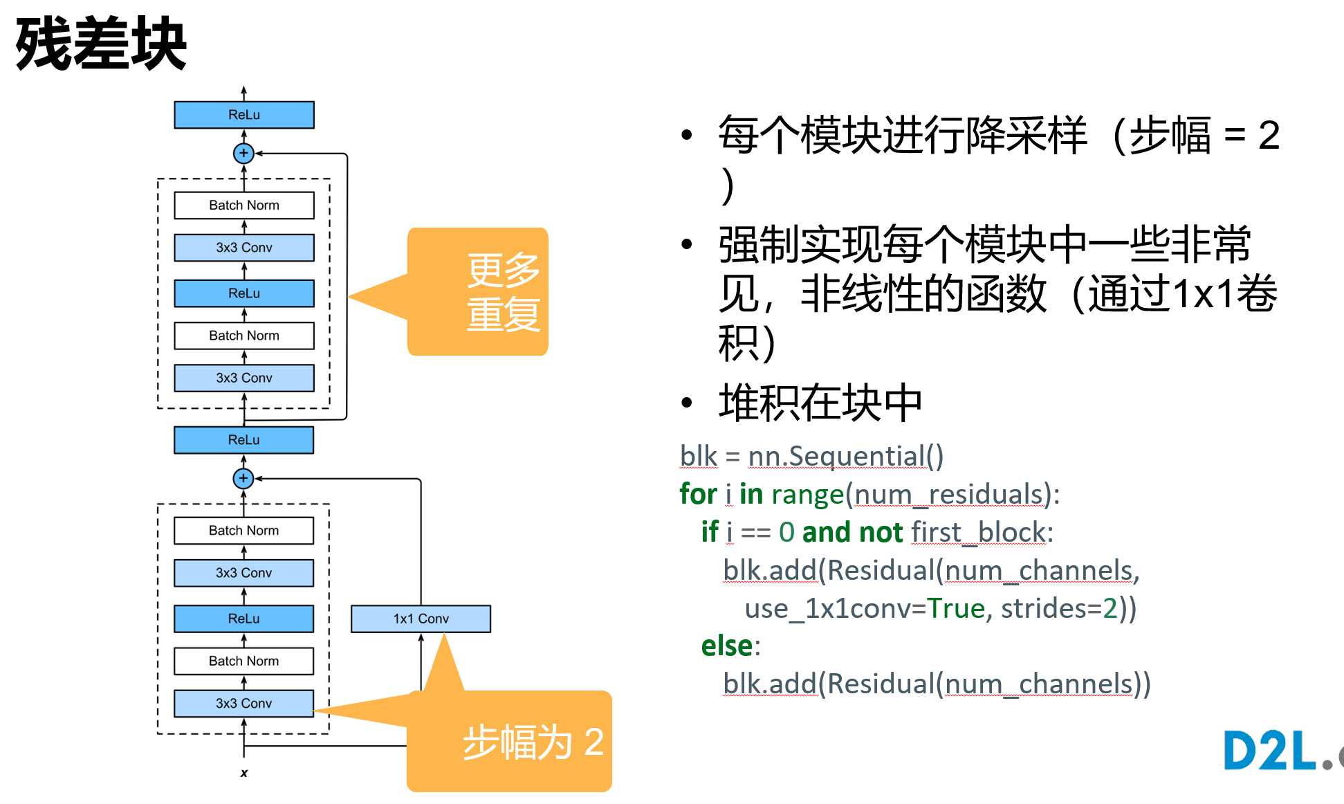
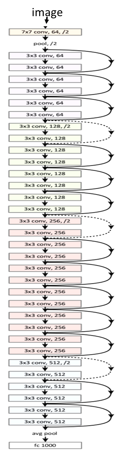
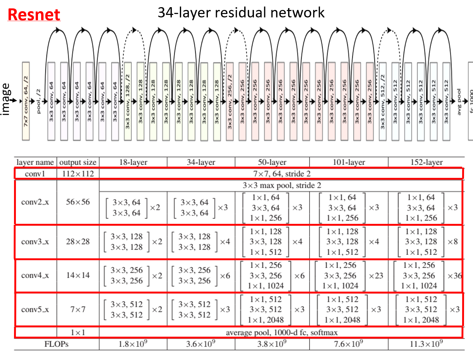
nn.Linear(84, 10))残差网络 ResNet
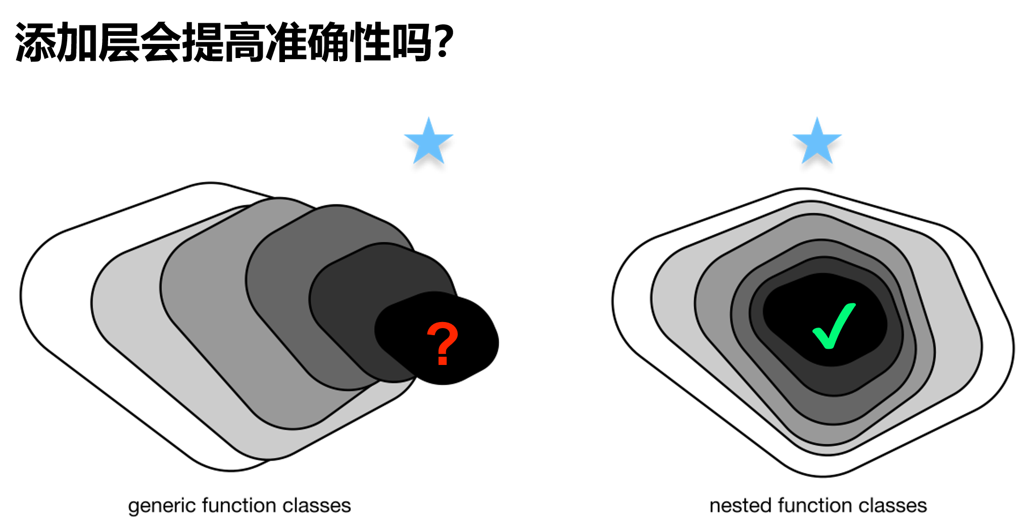
残差块具有两种结构,左面那个是输入输出通道不变的时候;右边那个是改变通道数的时候
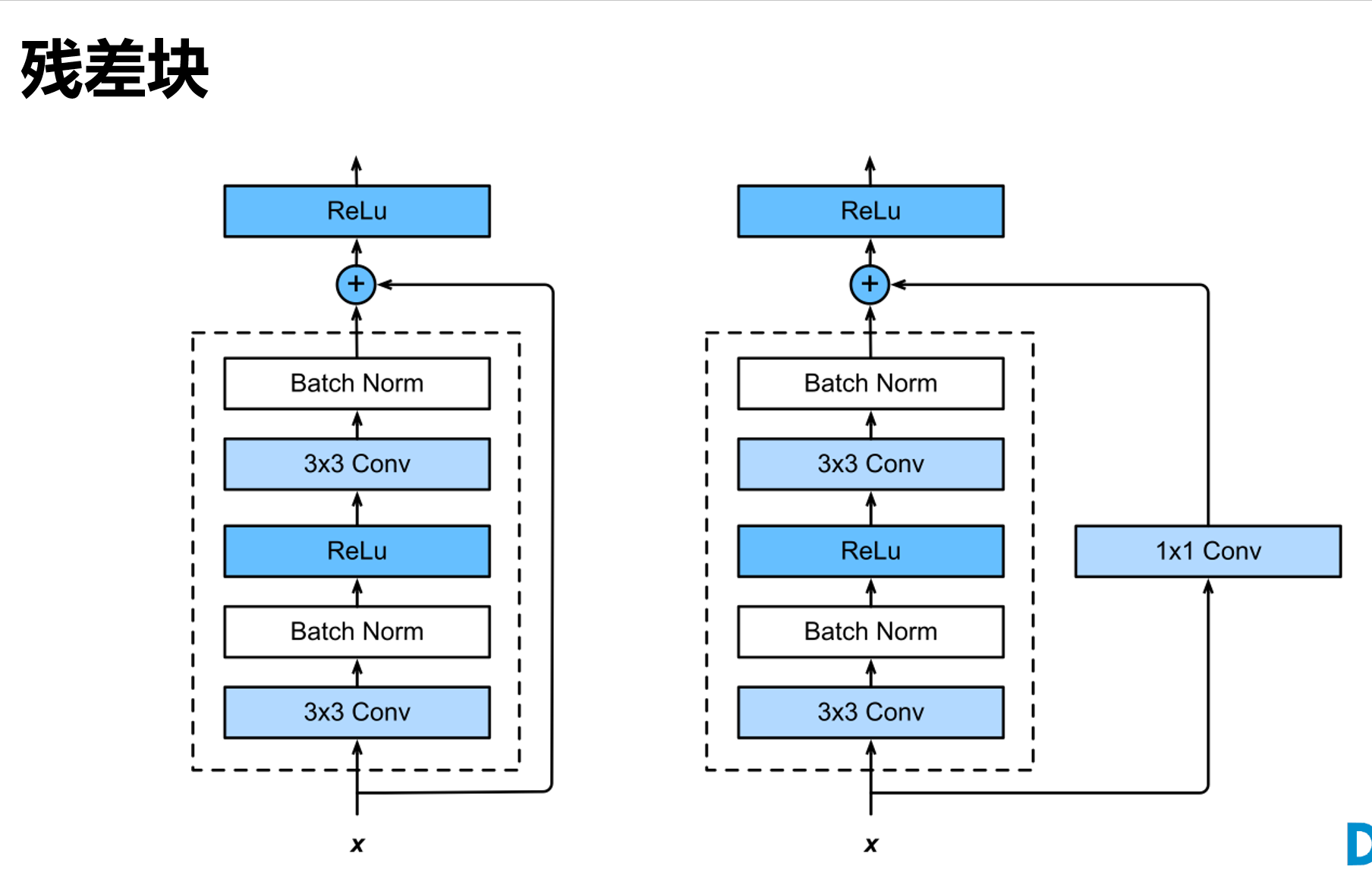
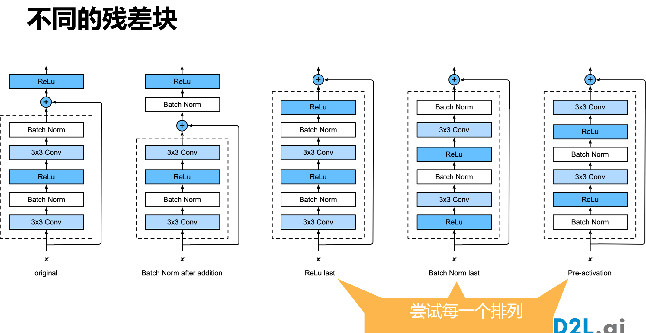
很多学者对残差结构进行了调整。何凯明等在获得竞赛大奖后,也对残差结构进行了优化:预激活 pre-activation,BN和ReLU都提前了,即上面图片最右边的结构和下面的图片所示结构。
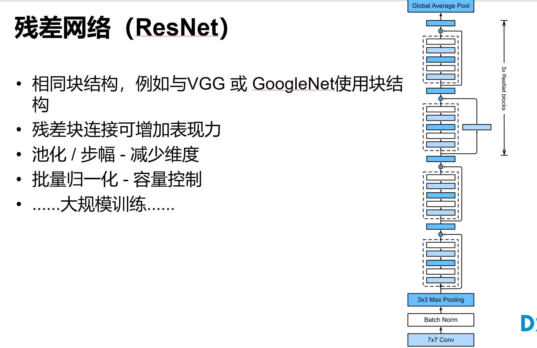
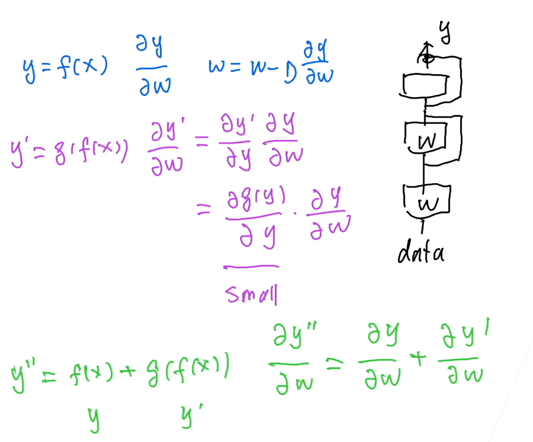
从梯度上将ResNet为什么work
加入g(x)为一个全连接层,对数据拟合效果比较好,那么它的梯度相应的会比较小,所以越往后,它的梯度越小。
但是用ResNet后,引入加法,使得后面层的梯度不至于过小。
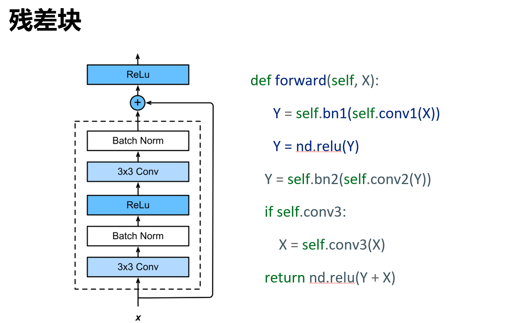
ResNet18代码
class Residual(nn.Module):
def __init__(self, input_channels, num_channels,
use_1x1conv=False, strides=1):
super().__init__()
self.conv1 = nn.Conv2d(input_channels, num_channels,
kernel_size=3, padding=1, stride=strides)
self.conv2 = nn.Conv2d(num_channels, num_channels,
kernel_size=3, padding=1)
if use_1x1conv:
self.conv3 = nn.Conv2d(input_channels, num_channels,
kernel_size=1, stride=strides)
else:
self.conv3 = None
self.bn1 = nn.BatchNorm2d(num_channels)
self.bn2 = nn.BatchNorm2d(num_channels)
def forward(self, X):
Y = F.relu(self.bn1(self.conv1(X)))
Y = self.bn2(self.conv2(Y))
if self.conv3:
X = self.conv3(X)
Y += X
return F.relu(Y)
class ResNet(nn.Module):
def __init__(self,in_channels) -> None:
super().__init__()
b1 = nn.Sequential(nn.Conv2d(in_channels, 64, kernel_size=7, stride=2, padding=3),
nn.BatchNorm2d(64), nn.ReLU(),
nn.MaxPool2d(kernel_size=3, stride=2, padding=1))
b2 = nn.Sequential(*ResNet.resnet_block(64, 64, 2, first_block=True))
b3 = nn.Sequential(*ResNet.resnet_block(64, 128, 2))
b4 = nn.Sequential(*ResNet.resnet_block(128, 256, 2))
b5 = nn.Sequential(*ResNet.resnet_block(256, 512, 2))
self.model = nn.Sequential(b1, b2, b3, b4, b5,
nn.AdaptiveAvgPool2d((1,1)),
nn.Flatten(), nn.Linear(512, 10))
@staticmethod
def resnet_block(input_channels, num_channels, num_residuals,
first_block=False):
blk = []
for i in range(num_residuals):
if i == 0 and not first_block:
blk.append(Residual(input_channels, num_channels,
use_1x1conv=True, strides=2))
else:
blk.append(Residual(num_channels, num_channels))
return blk
def forward(self,x):
return self.model(x)
def checkout_channel(self,X=None):
for blk in self.model:
X = blk(X)
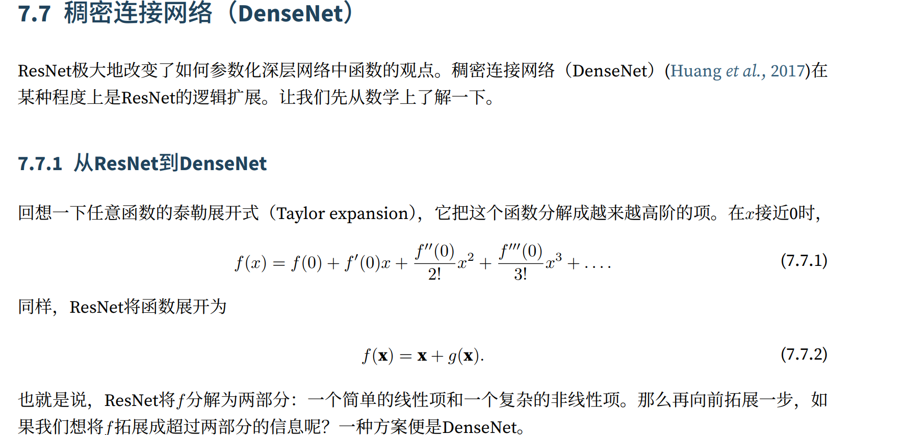
print(blk.__class__.__name__,'output shape:\t',X.shape)DenseNet
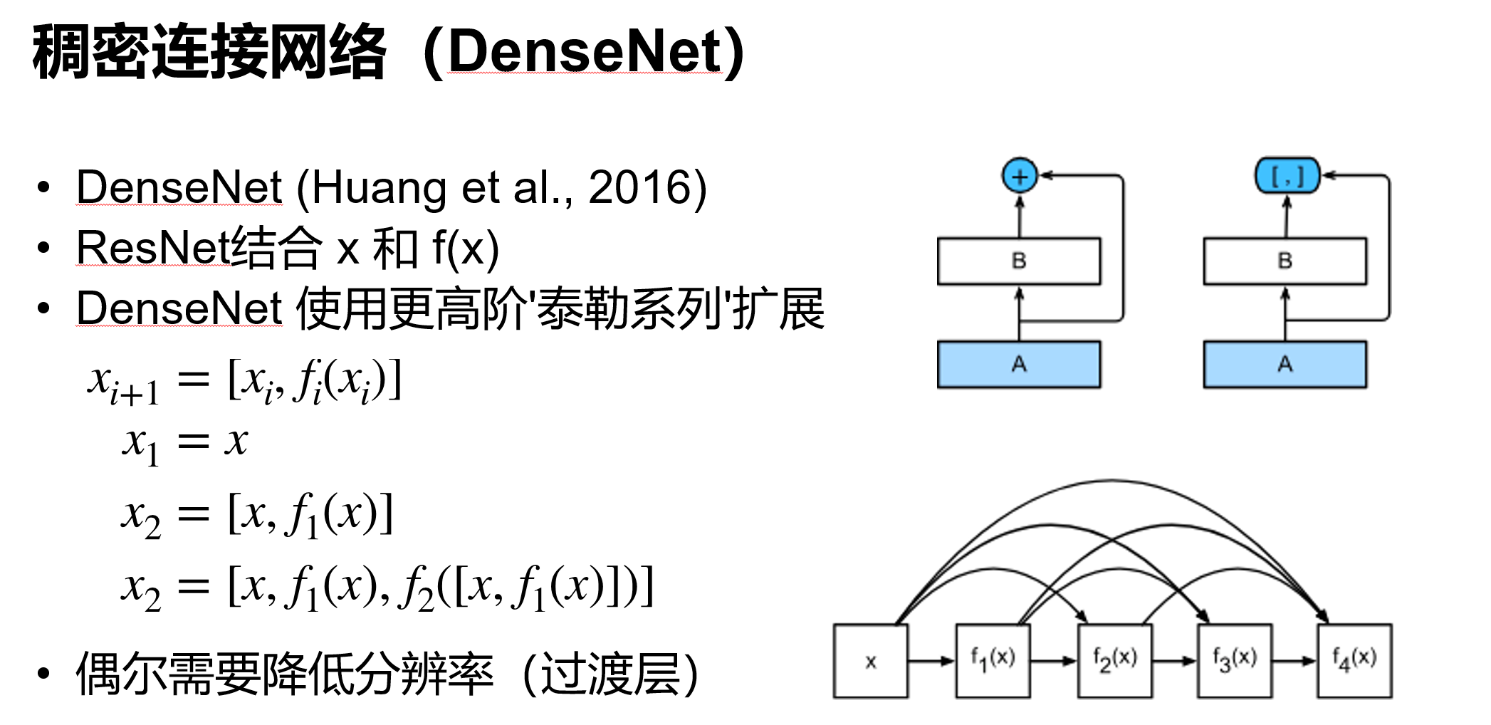
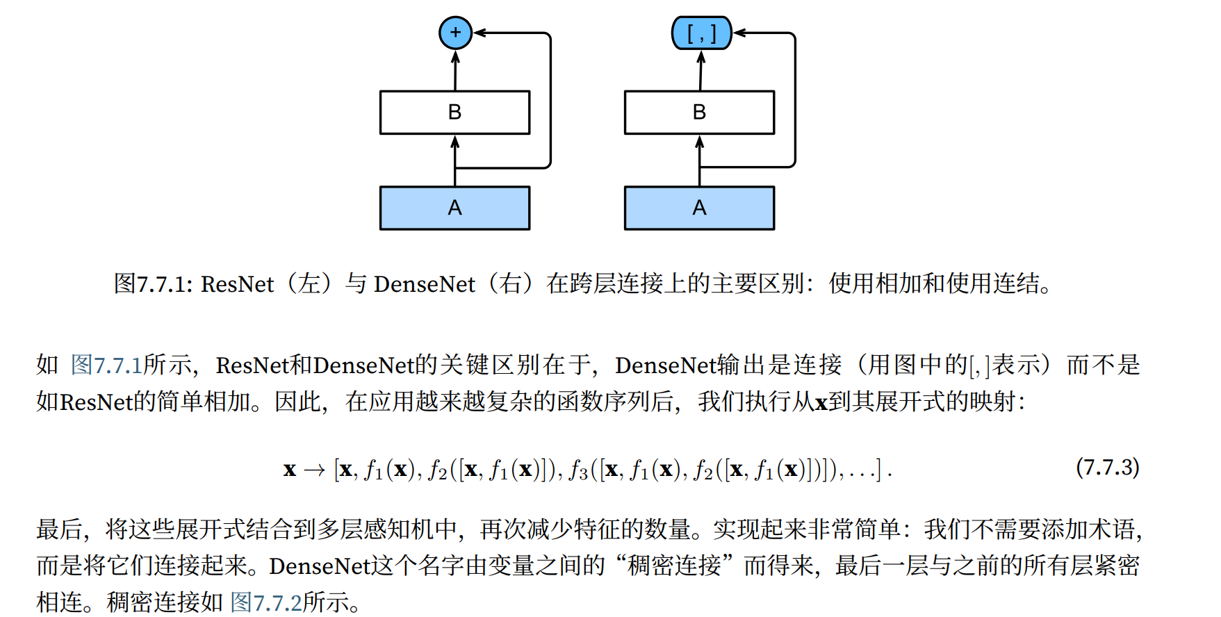
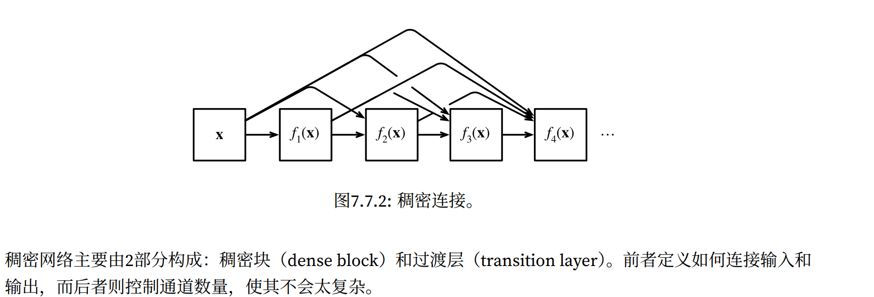
⼀个稠密块由多个卷积块组成,每个卷积块使⽤相同数量的输出通道。然⽽,在前向传播中,我们将每个卷
积块的输⼊和输出在通道维上连结。
import torch
from torch import nn
from d2l import torch as d2l


def conv_block(input_channels, num_channels):
    return nn.Sequential(
        nn.BatchNorm2d(input_channels), nn.ReLU(),
        nn.Conv2d(input_channels, num_channels, kernel_size=3, padding=1))

class DenseBlock(nn.Module):
    def __init__(self, num_convs, input_channels, num_channels):
        super(DenseBlock, self).__init__()
        layer = []
        for i in range(num_convs):
            layer.append(conv_block(
                num_channels * i + input_channels, num_channels))
        self.net = nn.Sequential(*layer)

    def forward(self, X):
        for blk in self.net:
            Y = blk(X)
            # # 连接通道维度上每个块的输⼊和输出
            X = torch.cat((X, Y), dim=1)
        return X
在下⾯的例⼦中,我们定义⼀个有2个输出通道数为10的DenseBlock。使⽤通道数为3的输⼊时,我们会得到
通道数为3 + 2 × 10 = 23的输出。卷积块的通道数控制了输出通道数相对于输⼊通道数的增⻓,因此也被称
为增⻓率(growth rate)。
blk = DenseBlock(2, 3, 10)
X = torch.randn(4, 3, 8, 8)
Y = blk(X)
Y.shape
# torch.Size([4, 23, 8, 8])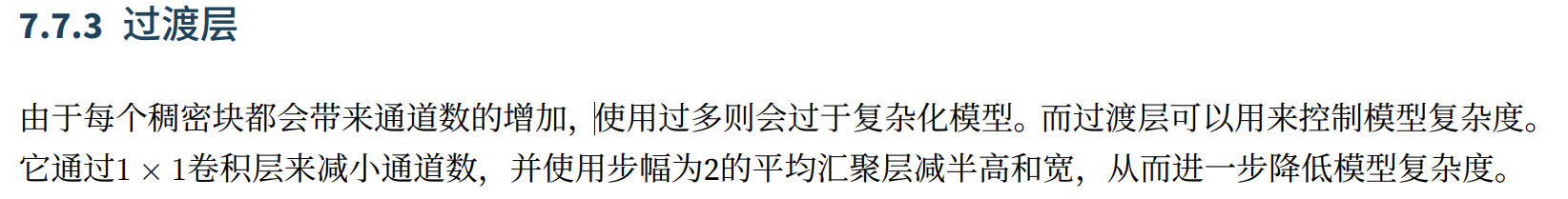
def transition_block(input_channels, num_channels):
    return nn.Sequential(
        nn.BatchNorm2d(input_channels), nn.ReLU(),
        nn.Conv2d(input_channels, num_channels, kernel_size=1),
        nn.AvgPool2d(kernel_size=2, stride=2))
blk = transition_block(23, 10)
blk(Y).shape
#torch.Size([4, 10, 4, 4])DenseNet模型
b1 = nn.Sequential(
    nn.Conv2d(1, 64, kernel_size=7, stride=2, padding=3),
    nn.BatchNorm2d(64), nn.ReLU(),
    nn.MaxPool2d(kernel_size=3, stride=2, padding=1))

num_channels, growth_rate = 64, 32
num_convs_in_dense_blocks = [4, 4, 4, 4]
blks = []
for i, num_convs in enumerate(num_convs_in_dense_blocks):
    blks.append(DenseBlock(num_convs, num_channels, growth_rate))
    num_channels += num_convs * growth_rate
    if i != len(num_convs_in_dense_blocks) - 1:
        blks.append(transition_block(num_channels, num_channels // 2))
        num_channels = num_channels // 2

net = nn.Sequential(
    b1, *blks,
    nn.BatchNorm2d(num_channels), nn.ReLU(),
    nn.AdaptiveAvgPool2d((1, 1)),
    nn.Flatten(),
    nn.Linear(num_channels, 10))
Squeeze-Excite Net(SENet)
ShuffleNet
CBAM
深度学习硬件:CPU 和 GPU
单机多卡并行
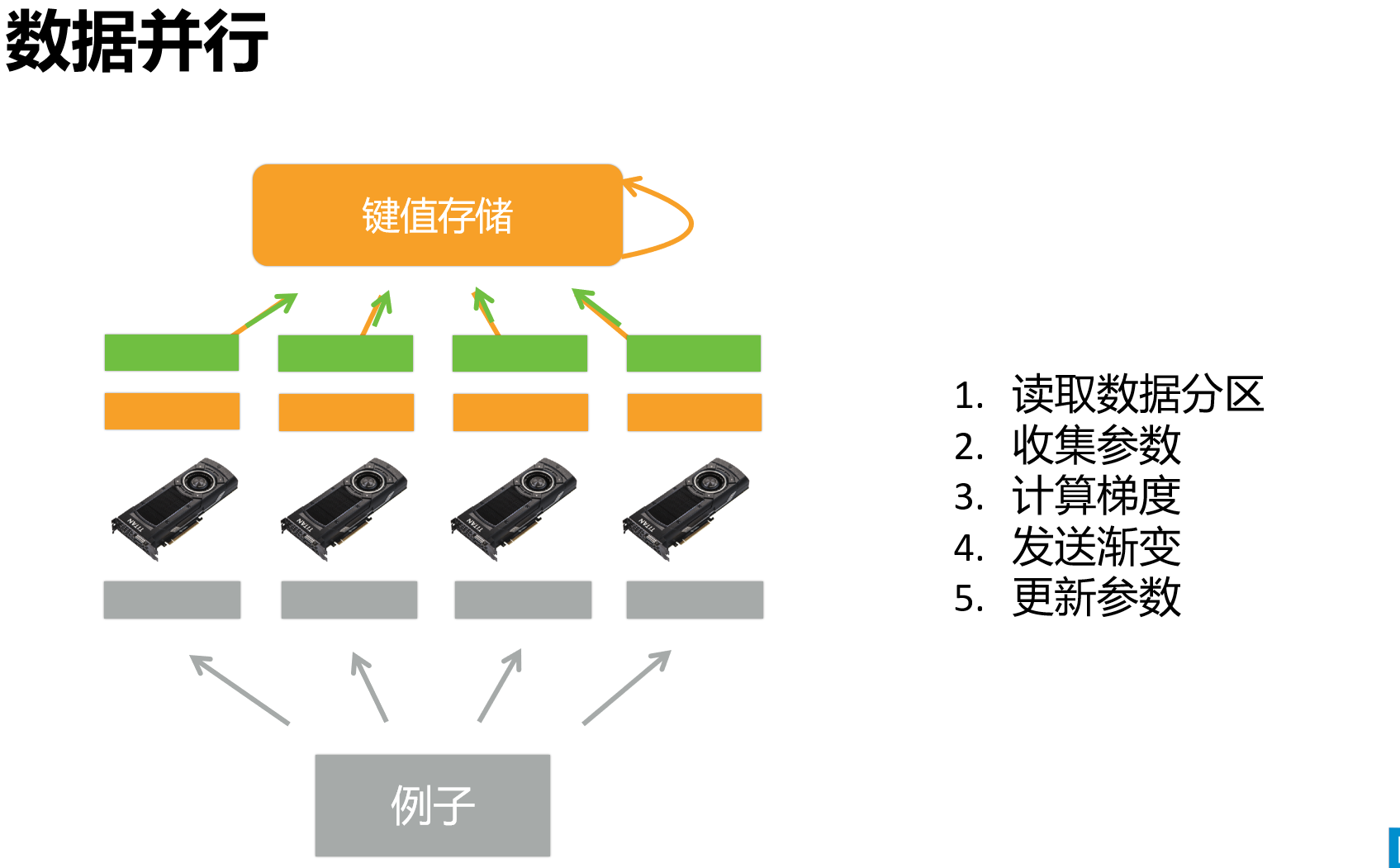
分布式训练
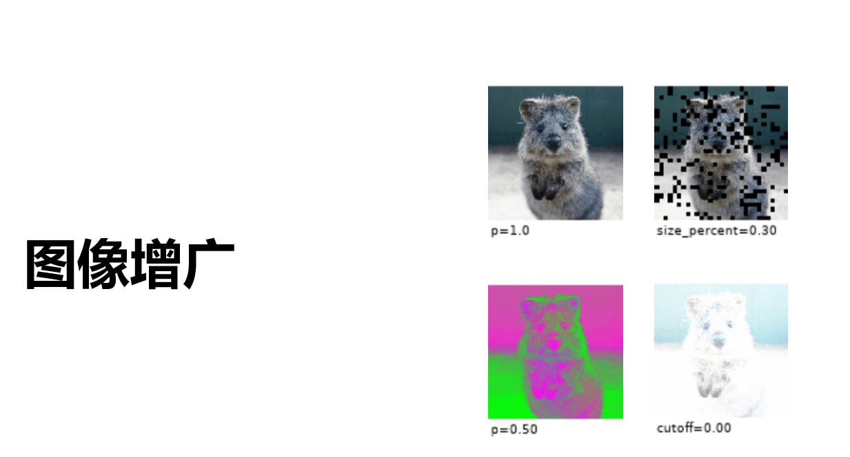
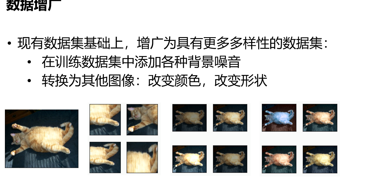
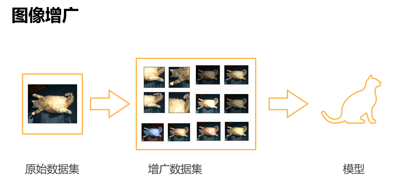
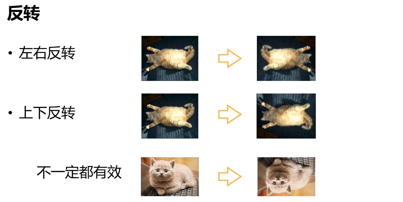
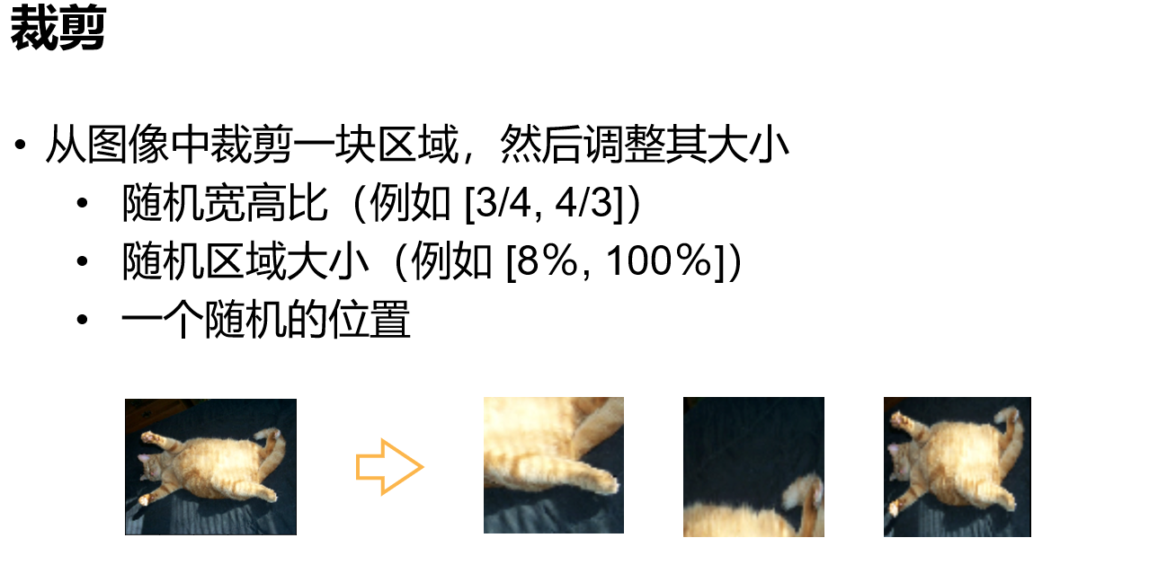
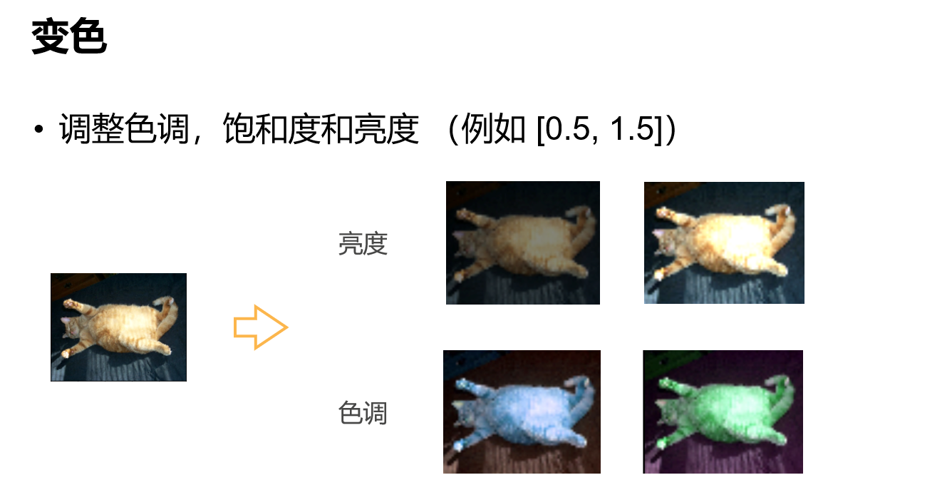
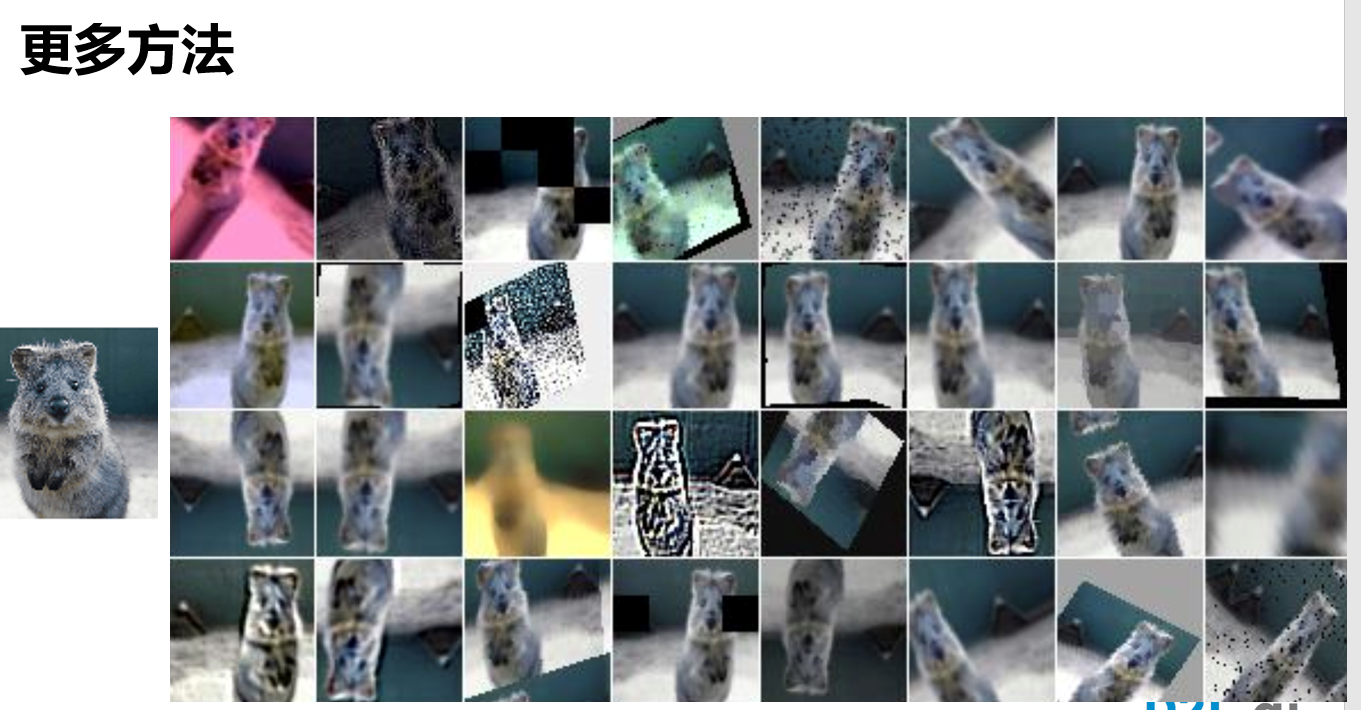
数据增广
确定需要什么样的数据增强,可以从后往前推,即分析测试集中的数据可能会是什么样的,然后选择合适的数据增强。可以近似的看做一个正则操作,降低过拟合,甚至有可能测试精度会高于训练精度

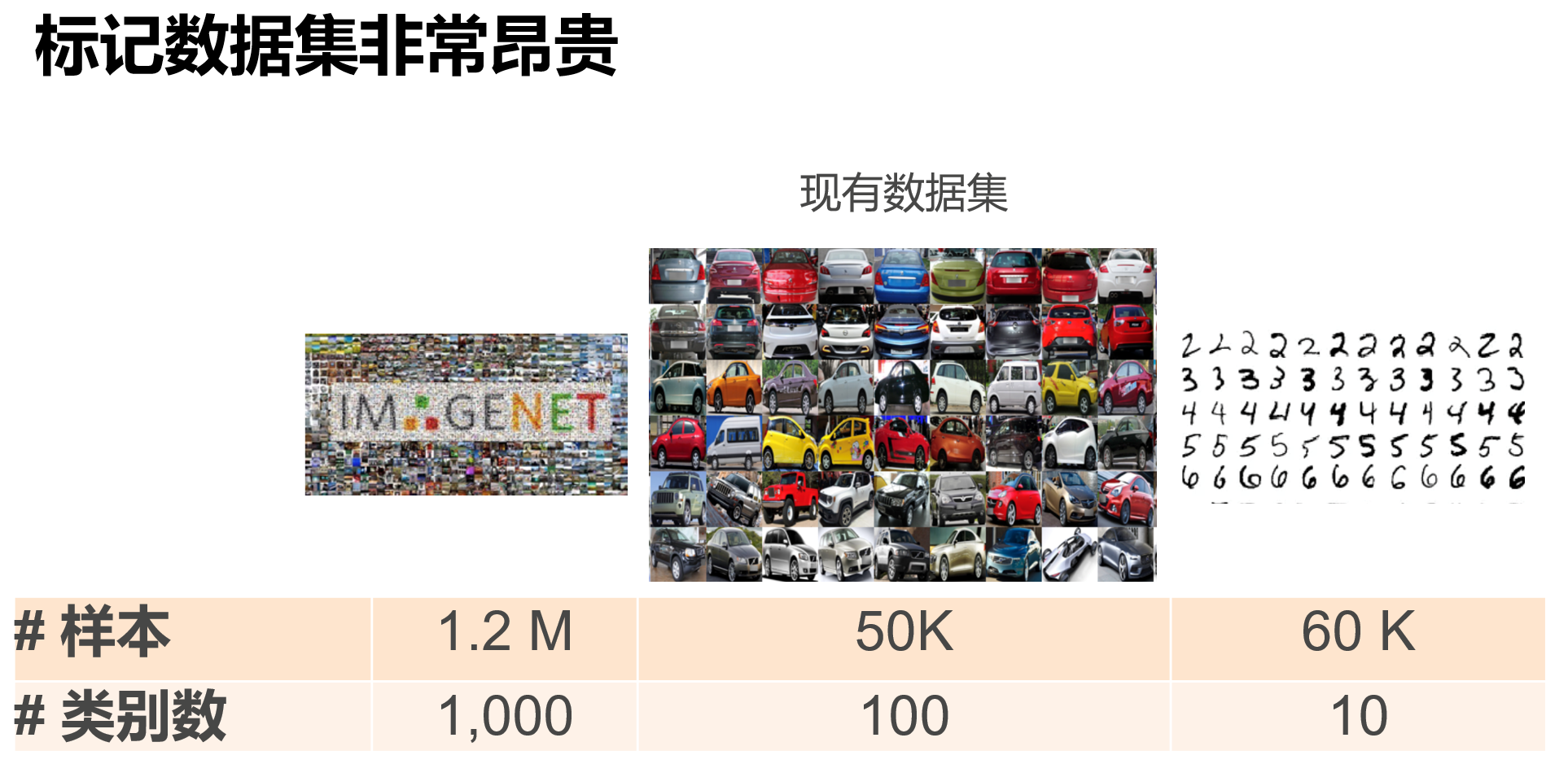
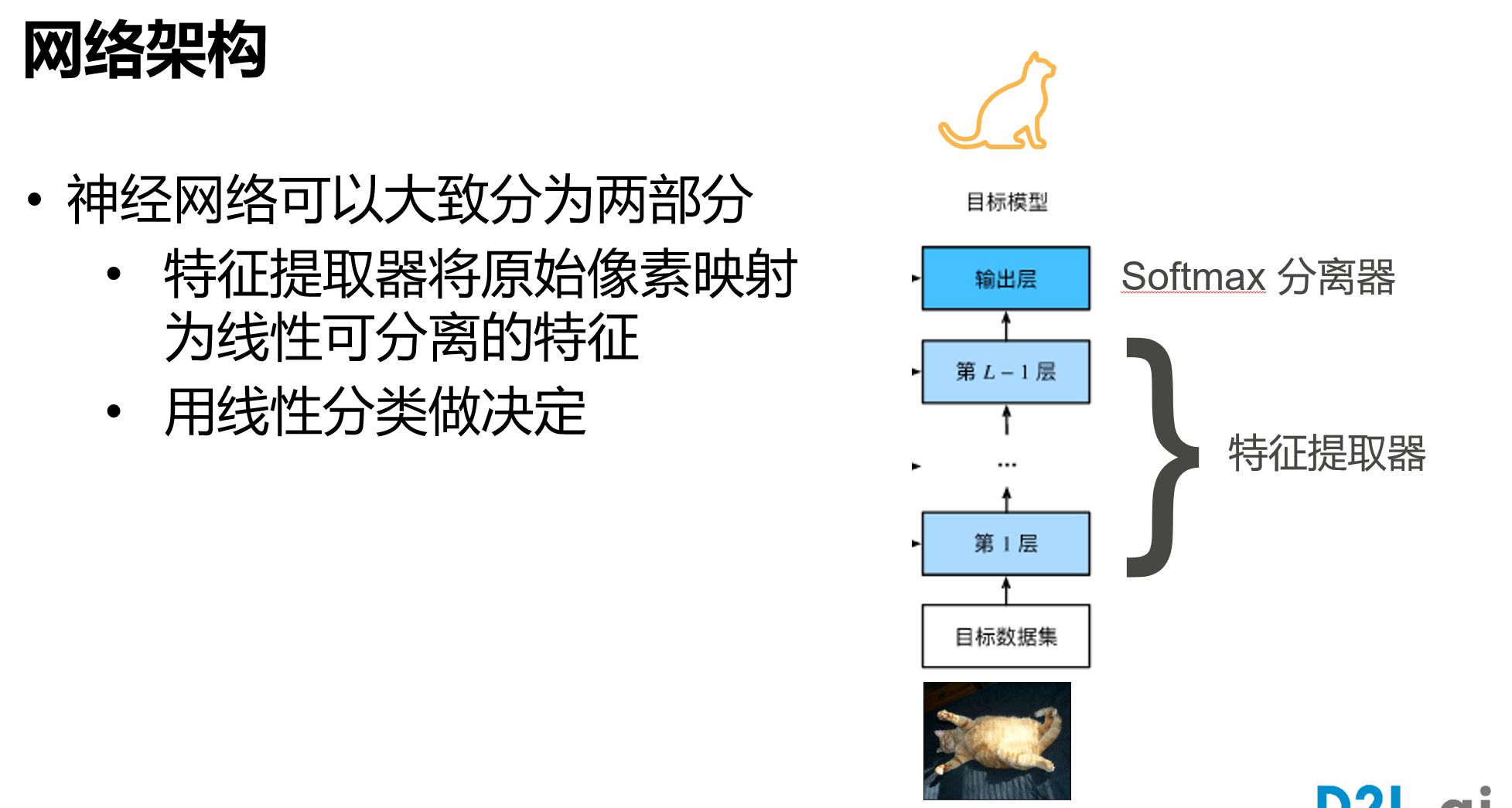
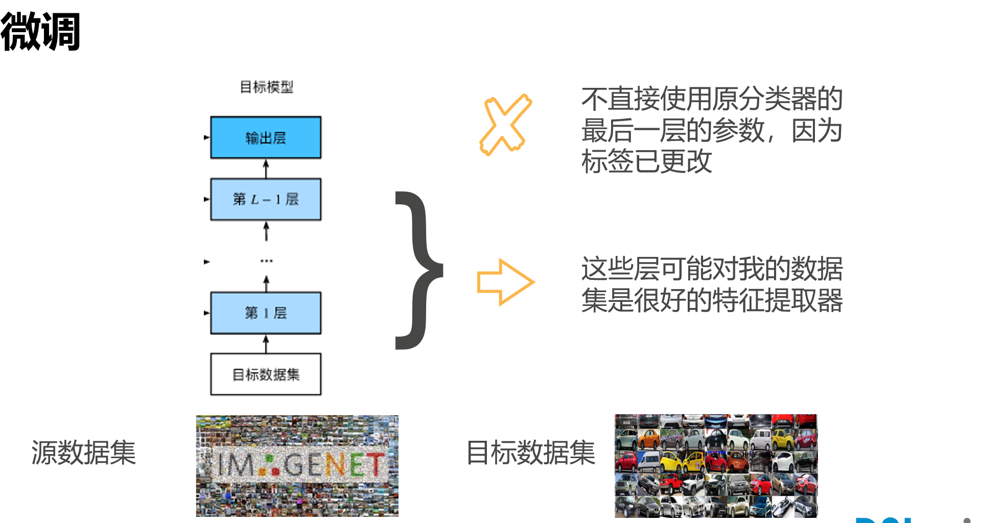
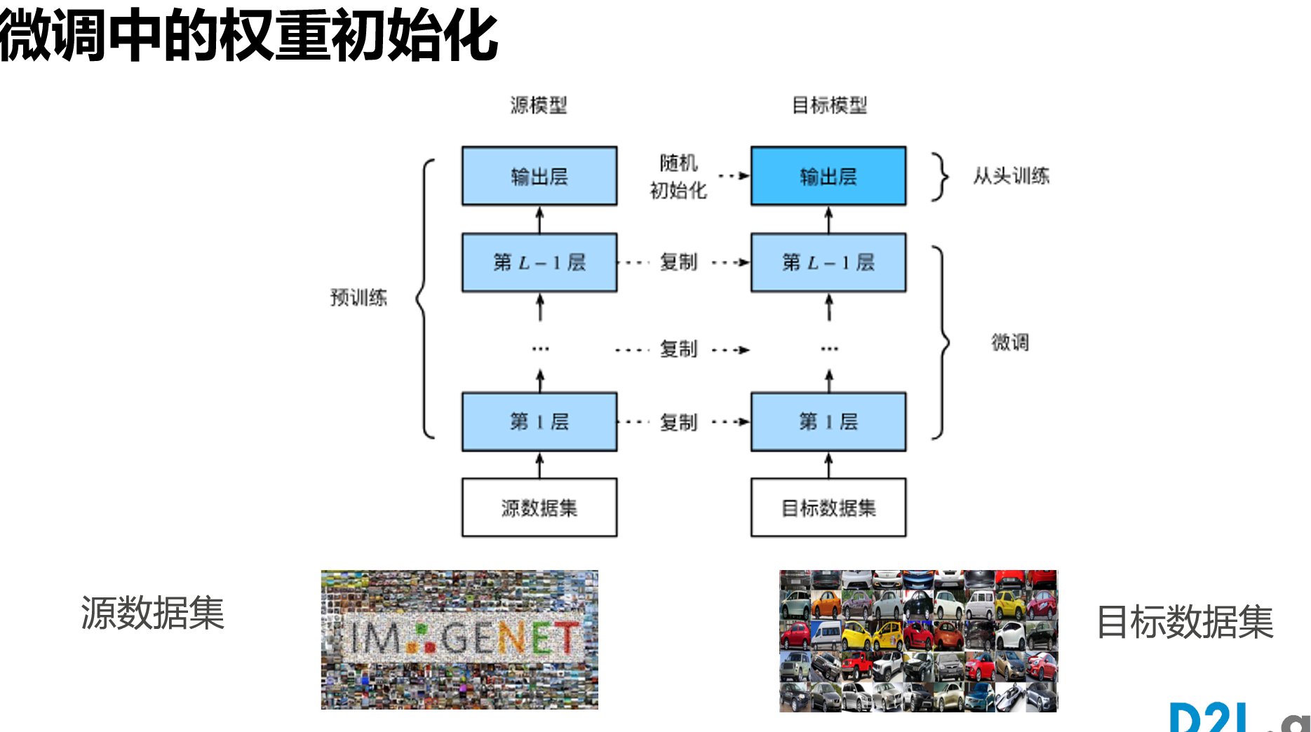
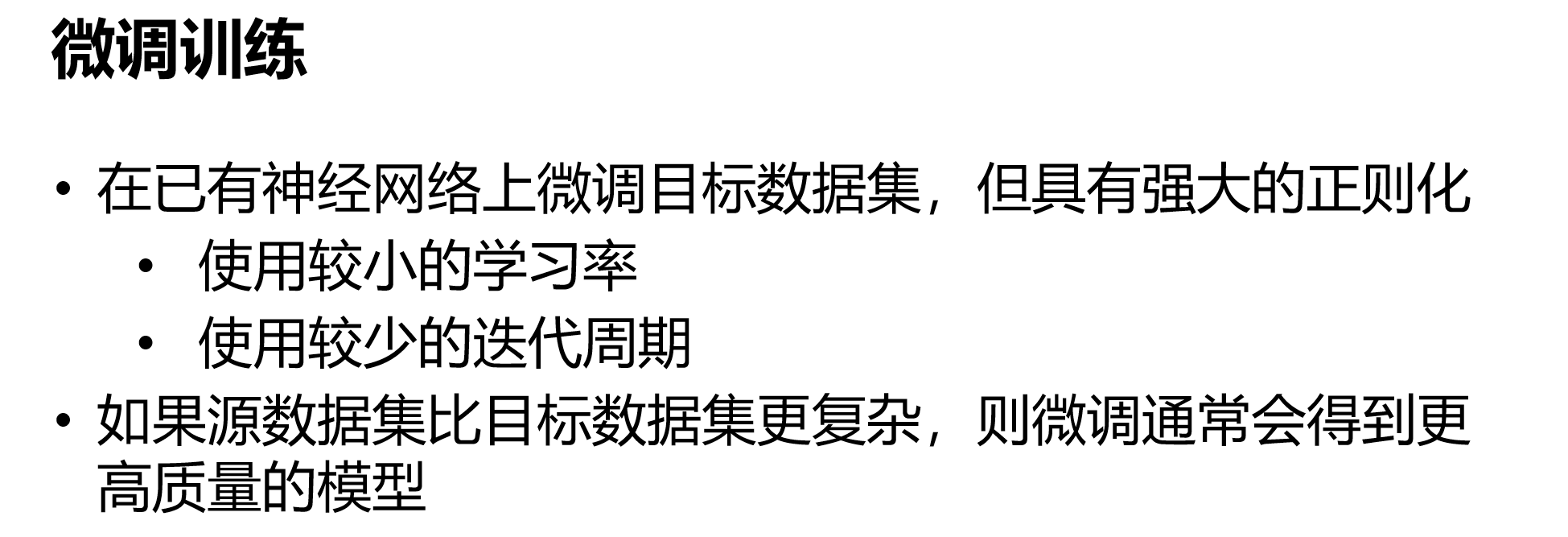
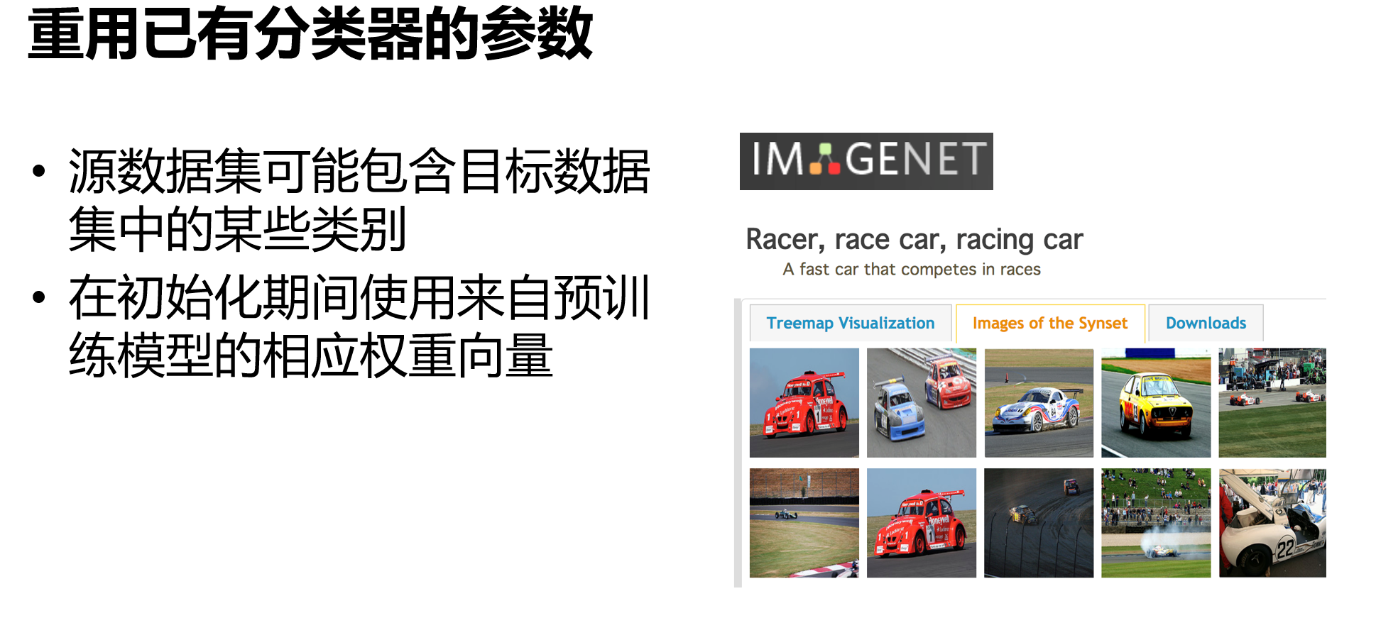
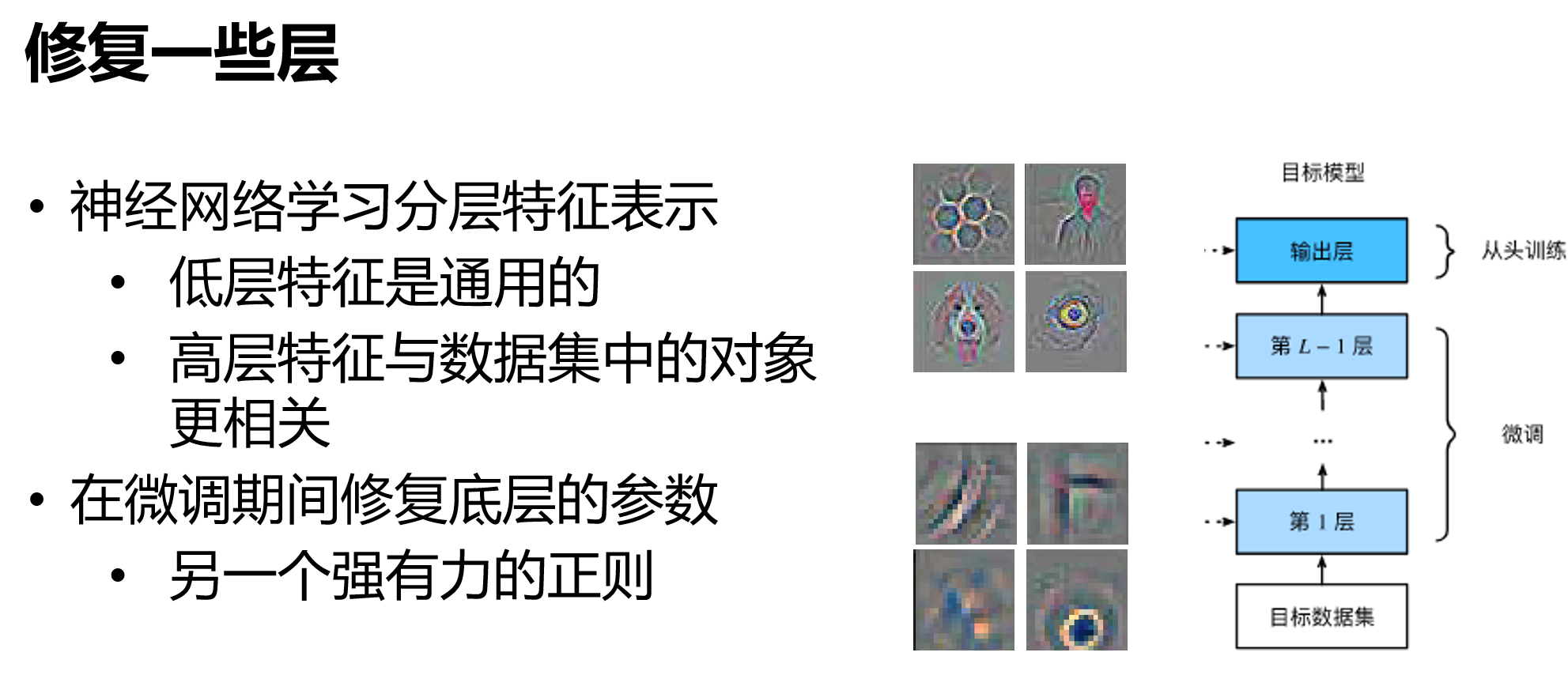
微调[很重要]
pretrained
迁移学习
源数据集和目标数据集要类似
目标检测
物体检测和数据集
调参总结
- batch size对训练集精度的影响比较大,batch size较小,可以更好的拟合训练集,训练精度越大;但是对测试集的精度基本没有影响。
- ReLU()效果确实比Sigmoid要好一些
沐言沐语
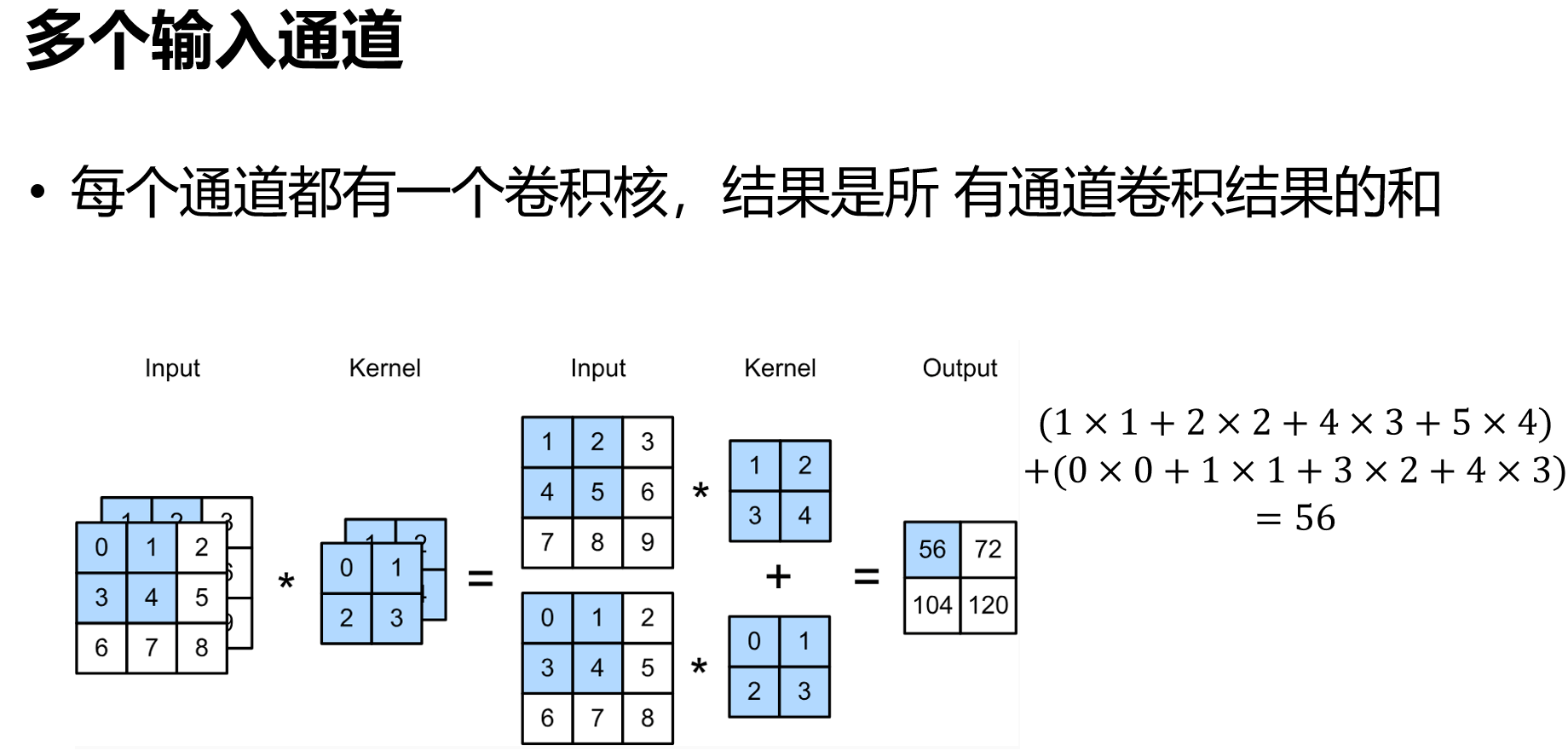
- 二维卷积指的输入的图片只考虑高和宽,不考虑channel。如果是深度图,就是额外多一个深度,可以用3D卷积
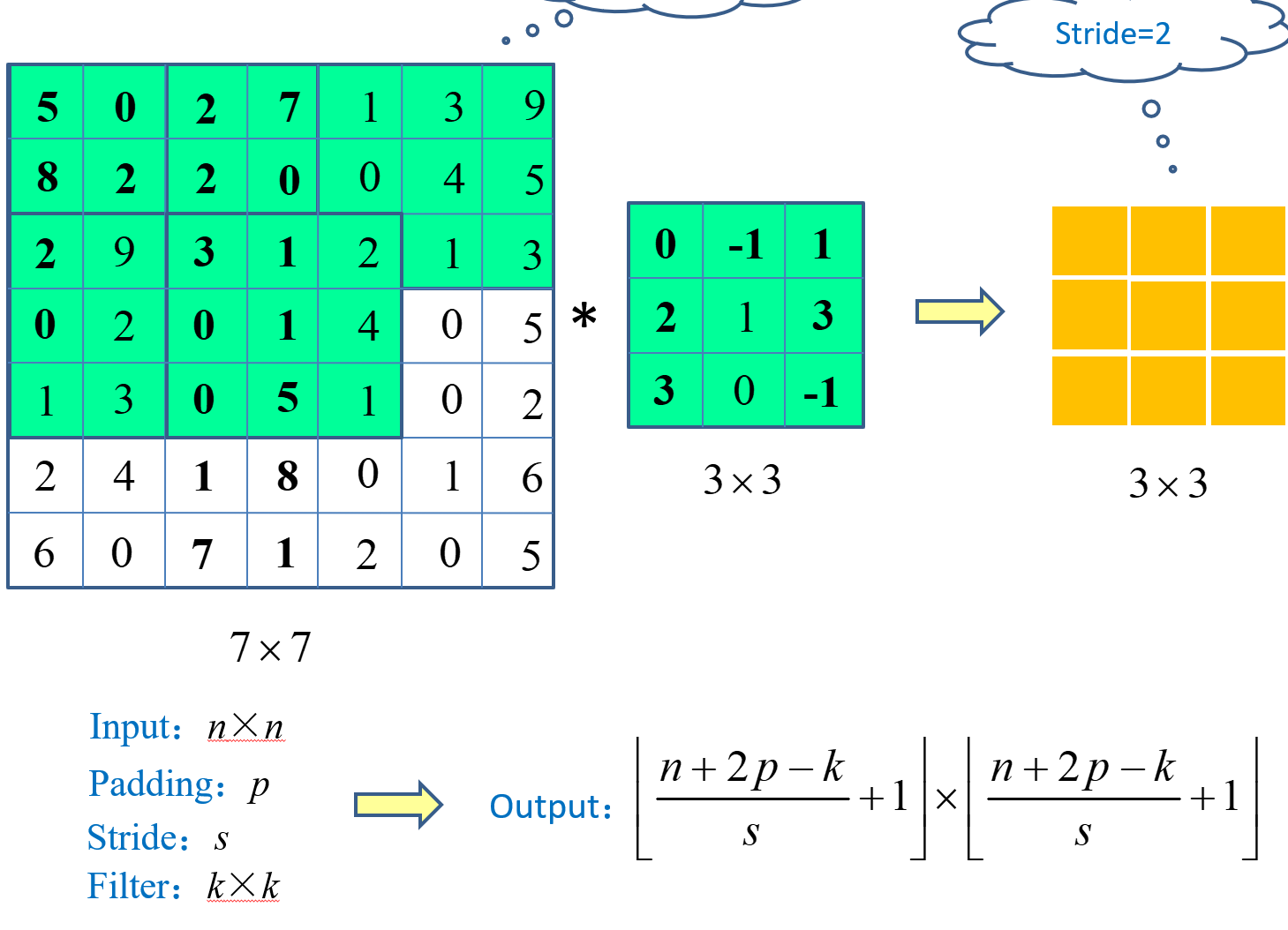
- 卷积操作,对于位置是非常敏感的,用池化操作消除这种影响
- 池化层一般放在卷积层后(消除卷积对于位置的敏感性),池化层目前用的越来越少了。池化可以1 消除卷积对于位置的敏感性 2 减少计算量 , 对于2 我们可以把stride放入卷积层中来减少计算量,对于1 我们现在常常做数据增强,来淡化卷积对于位置的敏感性
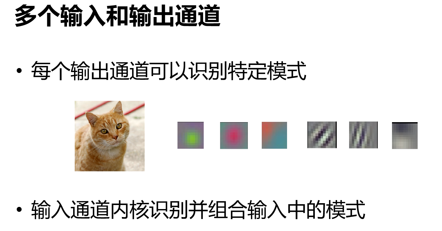
- 通过LeNet可以看出,卷积把高和宽不断减小,但是我们在这个过程中,让通道数不断增多,每一个通道可以看做空间的一个pattern(模式),然后通过MLP训练得到输出。(通常来说,高宽减半的时候,通道数会变为原来的两倍,但是也不能把输出通道调的太大,不然容易overfitting)
- 图片作为网络的输出时,图片的大小可能是随机的,不一定是输入要求的大小,一般不会直接resize,而是保持高宽比,从里面抠出一个方的,可以多抠几次,一般效果不会差很多。
- 尽量用简单的模型,不要过度设计
- 就是pytorch训练好后,模型怎么进行部署应用,c++的话可以试试libtorch(边缘计算的话推荐TensorRT)
- 在实际深度学习中,尽量不要微调经典网络中的结构,但是可以改变一下通道数,或者输入输出的大小
- 随着网络深度的增加,可以识别的pattern也增多,即通道数增多,但是,通道数太大容易overfitting,目前来看1024就已经差不多了
- BN会加速收敛(可以将lr调的比较大),但是对最后的精度基本没有提升。而且,BN一般用于网络比较深的时候,浅层MLP+BN效果可能没有那么好,用在激活函数之前
- 关于batch size大小,利用率gpu-util 到90%就行了。或者是增加batch size,来看每秒钟处理的样本数,如果增加到某一个大小,处理样本数增加不了很多的话就可以不用增加了。
- cos函数的学习率
- 训练acc不是一定大于测试acc,比如我们后面可能会在训练集中加入大量噪音或者做data argumentation,测试acc就有可能会大于训练acc
- 增加数据确实是提高泛发性最简单,最有效的方法。
- 不要过度调参,过度调参可能导致只fit到当前数据,泛化性不能保证,所以调参到一个相对还ok的结果就行了
- resnet18大概18M的样子,一个卷积层大概1M的样子
w -= lr*w.grad 和 w = w-lr*w.grad的区别- 能用矩阵就别写for-loop
- python 用多进程避免全局锁
- 想清楚你要干嘛,不然要学的东西那么多,怎么可能学的过来
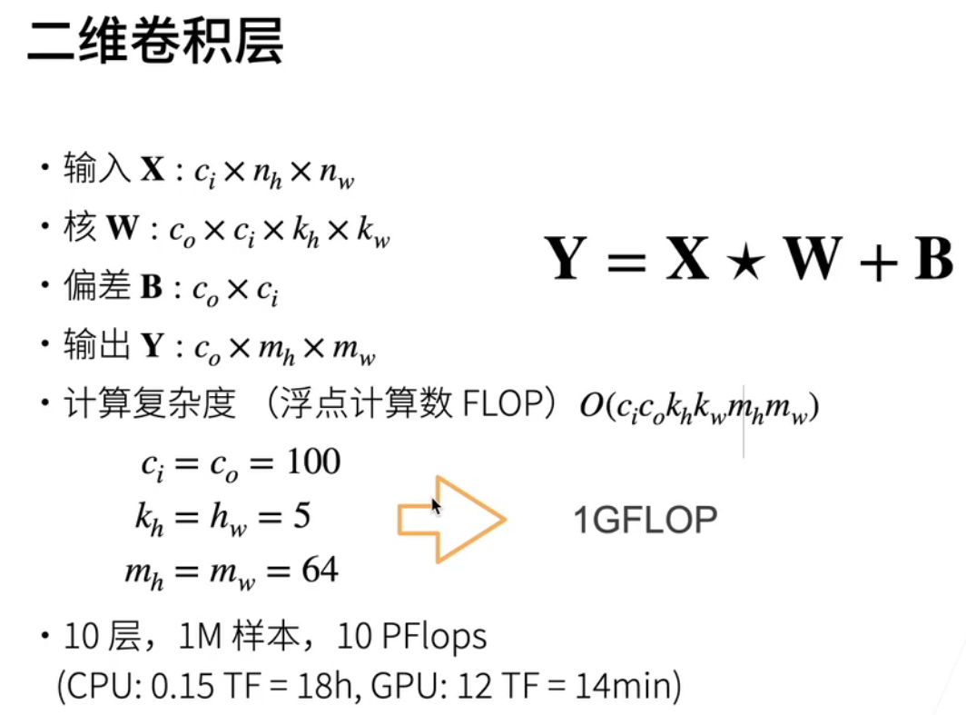
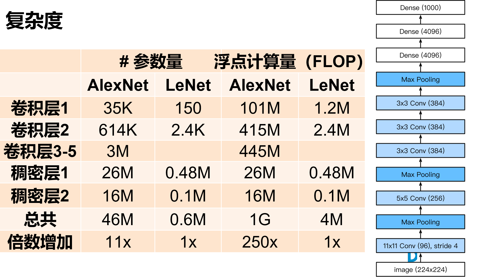
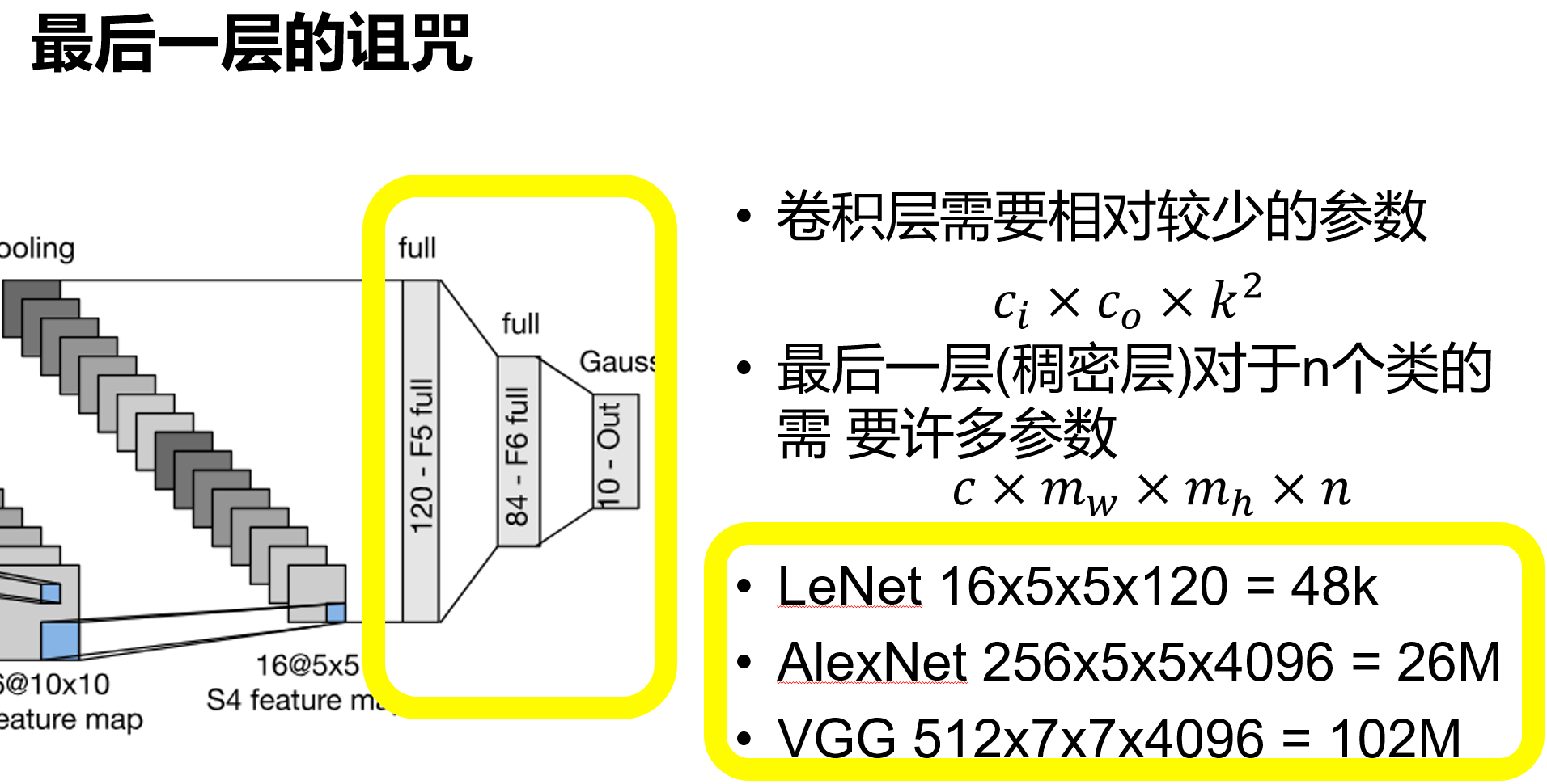
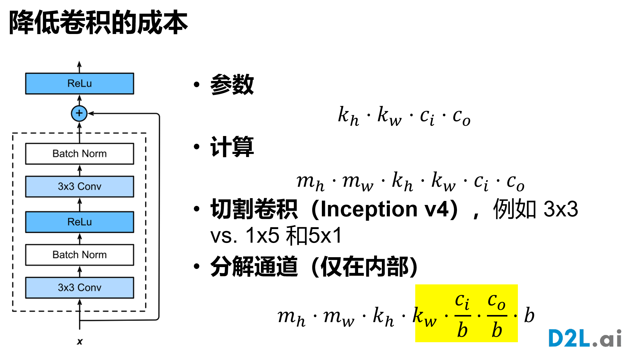
- 卷积的运算浮点数要远远大于全连接
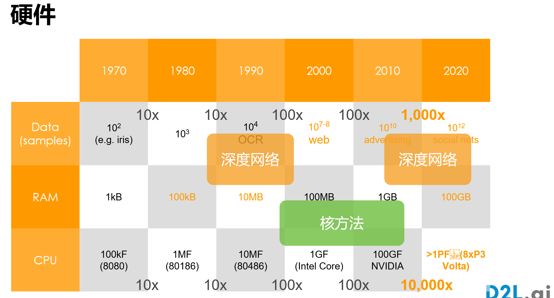
- 硬件 和 目前深度学习的发展,讨论鸡生蛋和蛋生鸡的问题,目前,确实是硬件shape深度学习。目前大模型和大数据离开不了硬件的发展。
- 多gpu训练,时间没变快是一件很常见的事,原因可能有1. data的读取花费大量的时间(有可能出现通讯开销大于计算开销) 2.虽然gpu增多了,但是你的数据批量大小没变,导致性能没有充分利用,要至少保证每个gpu的批量大小和之前单gpu时的批量大小一样,注意这时候测试精度可能会变低,要适当地调整学习率(增大)【batich size 和 lr两个因素控制了测试精度】,数据集多样性不够大的时候,不能用特别大的batch size,3.框架对并行的处理不够好(pytorch)4. 神经网络太小,导致数据并行没有明显优势 5.看看机器有没有别人在用
- 模型性能 看计算量(flops)和内存访问的比率,这个比率越高越好。往往参数比较小,算力比较高的模型性能高,比如卷积性能还不错,矩阵乘法也还可以
- 关于batch size大小的设置,和数据多样性、算法模型等都是有关的,一般分类的话有$n$个类,那么batch size大小在$10\cdot n$这个量级上
- 有时候发现其他的优化算法好像还没有SGD效果好,因为SGD做了很强的正则,有很多噪音在里面。
- 工业进行目标检测时,如果数据集小,可以进行迁移学习,把一个在很大数据集上训练好的模型拿过来
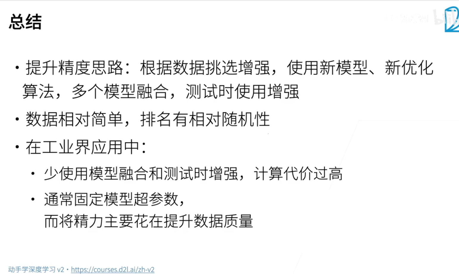
- 在图像分类任务而言,不用那么的追求高精度,95%已经够用了。工业实际与打比赛的要求确实不一样,工业更多专注数据质量(数据每天都在变化),打比赛是调模型(因为是死数据),工业是85%精度可以部署测试,然后不断增强数据质量,不断喂大量数据,基本3个月-半年后,模型基本可以达到95%以上是没问题的,然后部署生产环境,闭环落地!
附录
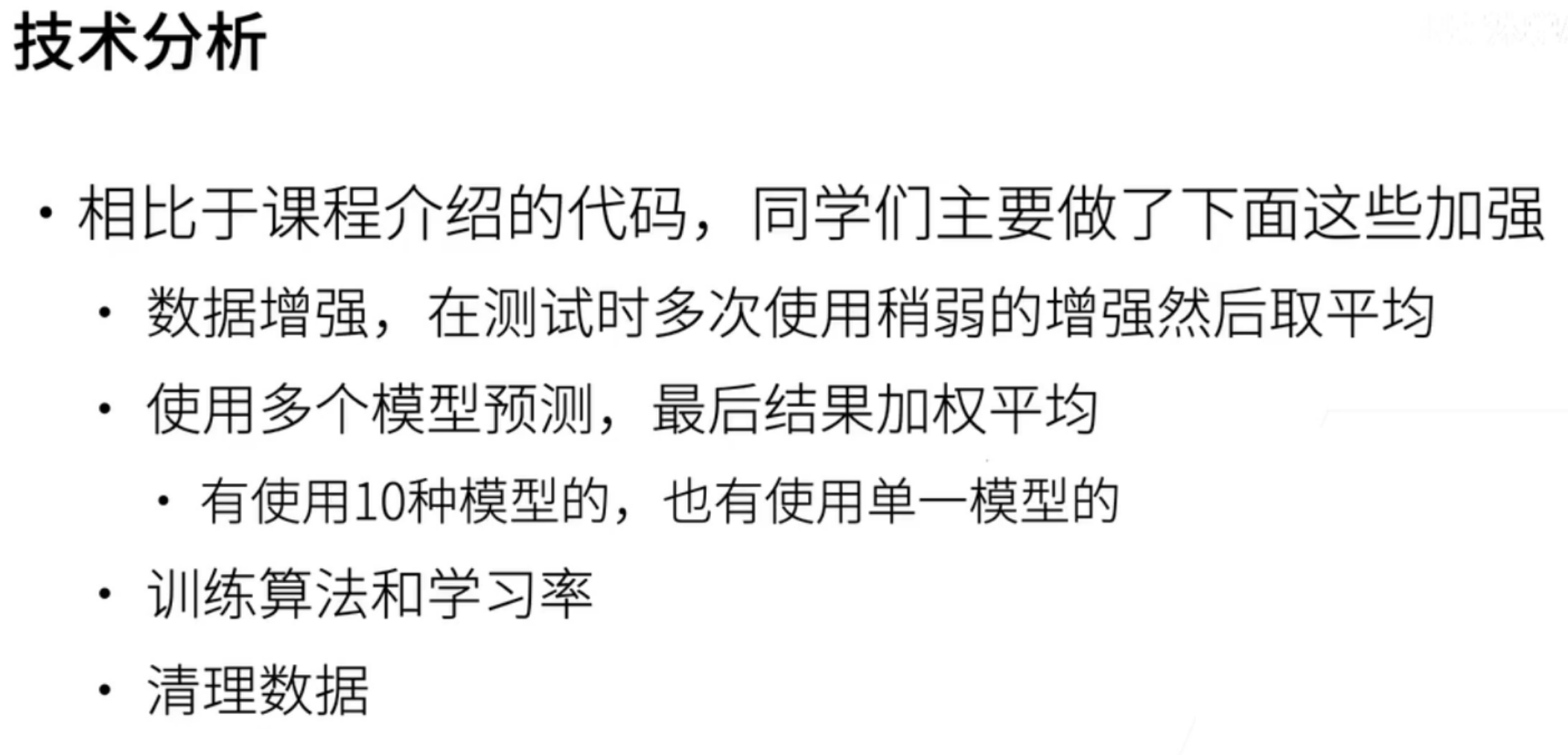
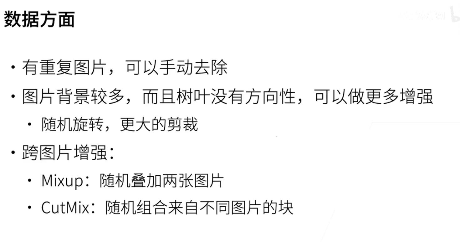
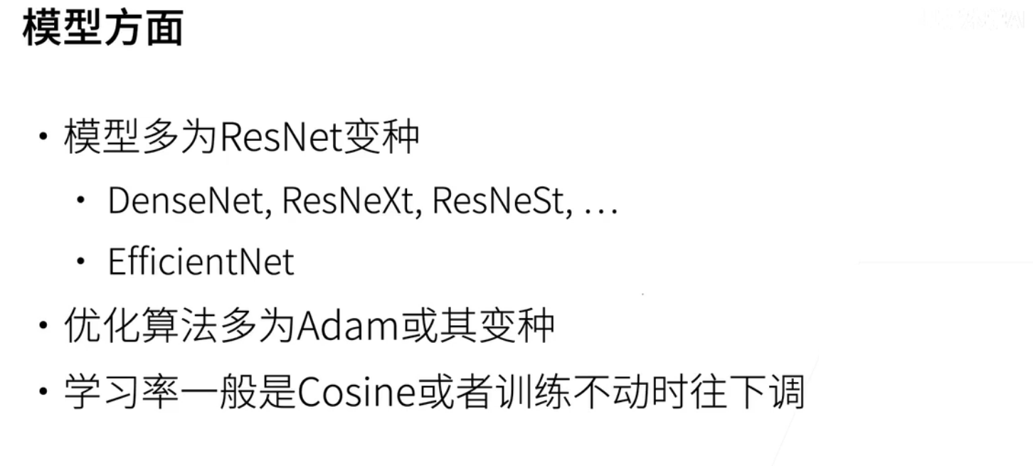
叶子竞赛